Function Level Profiling

Overview

Questions

• When is function level profiling appropriate?
• How can cProfile and snakeviz be used to profile a Python program?
• How are the outputs from function level profiling interpreted?

Objectives

• execute a Python program via cProfile to collect profiling information about a Python program’s execution
• use snakeviz to visualise profiling information output by cProfile
• interpret snakeviz views, to identify the functions where time is being spent during a program’s execution

Introduction

---

Software is typically comprised of a hierarchy of function calls, both functions written by the developer and those used from the language’s standard library and third party packages.

Function-level profiling analyses where time is being spent with respect to functions. Typically function-level profiling will calculate the number of times each function is called and the total time spent executing each function, inclusive and exclusive of child function calls.

This allows functions that occupy a disproportionate amount of the total runtime to be quickly identified and investigated.

In this episode we will cover the usage of the function-level profiler cProfile, how it’s output can be visualised with snakeviz and how the output can be interpreted.

What is a Call Stack?

The call stack keeps track of the active hierarchy of function calls and their associated variables.

As a stack it is a last-in first-out (LIFO) data structure.

A diagram of a call stack

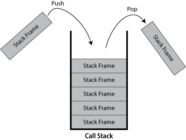
When a function is called, a frame to track it’s variables and metadata is pushed to the call stack. When that same function finishes and returns, it is popped from the stack and variables local to the function are dropped.

If you’ve ever seen a stack overflow error, this refers to the call stack becoming too large. These are typically caused by recursive algorithms, whereby a function calls itself, that don’t exit early enough.

Within Python the current call-stack can be printed using the core traceback package, traceback.print_stack() will print the current call stack.

The below example:

PYTHON

import traceback

def a():
    b1()
    b2()
def b1():
    pass
def b2():
    c()
def c():
    traceback.print_stack()

a()

Here we can see that the printing of the stack trace is called in c(), which is called by b2(), which is called by a(), which is called from global scope.

Hence, this prints the following call stack:

OUTPUT

  File "C:\call_stack.py", line 13, in <module>
    a()
  File "C:\call_stack.py", line 5, in a
    b2()
  File "C:\call_stack.py", line 9, in b2
    c()
  File "C:\call_stack.py", line 11, in c
    traceback.print_stack()

The first line states the file and line number where a() was called from (the last line of code in the file shown). The second line states that it was the function a() that was called, this could include it’s arguments. The third line then repeats this pattern, stating the line number where b2() was called inside a(). This continues until the call to traceback.print_stack() is reached.

You may see stack traces like this when an unhandled exception is thrown by your code.

In this instance the base of the stack has been printed first, other visualisations of call stacks may use the reverse ordering.

cProfile

---

cProfile is a function-level profiler provided as part of the Python standard library.

It can be called directly within your Python code as an imported package, however it’s easier to use it’s script interface:

SH

python -m cProfile -o <output file> <script name> <arguments>

For example if you normally run your program as:

SH

python my_script.py input.csv

You would call cProfile to produce profiling output out.prof with:

SH

python -m cProfile -o out.prof my_script.py input.csv

No additional changes to your code are required, it’s really that simple!

If you instead, don’t specify output to file (e.g. remove -o out.prof from the command), cProfile will produce output to console similar to that shown below:

OUTPUT

         28 function calls in 4.754 seconds

   Ordered by: standard name

   ncalls  tottime  percall  cumtime  percall filename:lineno(function)
        1    0.000    0.000    4.754    4.754 worked_example.py:1(<module>)
        1    0.000    0.000    1.001    1.001 worked_example.py:13(b_2)
        3    0.000    0.000    1.513    0.504 worked_example.py:16(c_1)
        3    0.000    0.000    1.238    0.413 worked_example.py:19(c_2)
        3    0.000    0.000    0.334    0.111 worked_example.py:23(d_1)
        1    0.000    0.000    4.754    4.754 worked_example.py:3(a_1)
        3    0.000    0.000    2.751    0.917 worked_example.py:9(b_1)
        1    0.000    0.000    4.754    4.754 {built-in method builtins.exec}
       11    4.753    0.432    4.753    0.432 {built-in method time.sleep}
        1    0.000    0.000    0.000    0.000 {method 'disable' of '_lsprof.Profiler' objects}

The columns have the following definitions:

Column	Definition
ncalls	The number of times the given function was called.
tottime	The total time spent in the given function, excluding child function calls.
percall	The average tottime per function call (tottime/ncalls).
cumtime	The total time spent in the given function, including child function calls.
percall	The average cumtime per function call (cumtime/ncalls).
filename:lineno(function)	The location of the given function’s definition and it’s name.

This output can often exceed the terminal’s buffer length for large programs and can be unwieldy to parse, so the package snakeviz is often utilised to provide an interactive visualisation of the data when exported to file.

snakeviz

---

snakeviz is a web browser based graphical viewer for cProfile output files. It is not part of the Python standard library, and therefore must be installed via pip.

SH

pip install snakeviz

Once installed, you can visualise a cProfile output file such as out.prof via:

SH

python -m snakeviz out.prof

This should open your web browser displaying a page similar to that below.

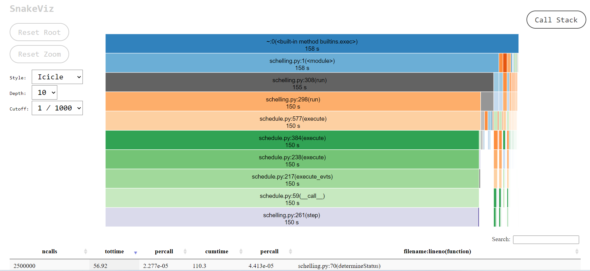
An example of the default ‘icicle’ visualisation provided by snakeviz.

The icicle diagram displayed by snakeviz represents an aggregate of the call stack during the execution of the profiled code. The box which fills the top row represents the the root call, filling the row shows that it occupied 100% of the runtime. The second row holds the child methods called from the root, with their widths relative to the proportion of runtime they occupied. This continues with each subsequent row, however where a method only occupies 50% of the runtime, it’s children can only occupy a maximum of that runtime hence the appearance of “icicles” as each row gets narrower when the overhead of methods with no further children is accounted for.

By clicking a box within the diagram, it will “zoom” making the selected box the root allowing more detail to be explored. The diagram is limited to 10 rows by default (“Depth”) and methods with a relatively small proportion of the runtime are hidden (“Cutoff”).

As you hover each box, information to the left of the diagram updates specifying the location of the method and for how long it ran.

snakeviz Inside Notebooks

If you’re more familiar with writing Python inside Jupyter notebooks you can still use snakeviz directly from inside notebooks using the notebooks “magic” prefix (%) and it will automatically call cProfile for you.

First snakeviz must be installed and it’s extension loaded.

PY

!pip install snakeviz
%load_ext snakeviz

Following this, you can either call %snakeviz to profile a function defined earlier in the notebook.

PY

%snakeviz my_function()

Or, you can create a %%snakeviz cell, to profile the python executed within it.

PY

%%snakeviz

def my_function():
    print("Hello World!")

my_function()

In both cases, the full snakeviz profile visualisation will appear as an output within the notebook!

You may wish to right click the top of the output, and select “Disable Scrolling for Outputs” to expand it’s box if it begins too small.

Worked Example

---

To more clearly demonstrate how an execution hierarchy maps to the icicle diagram, the below toy example Python script has been implemented.

PYTHON

import time

def a_1():
    for i in range(3):
        b_1()
    time.sleep(1)
    b_2()
    
def b_1():
    c_1()
    c_2()

def b_2():
    time.sleep(1)
    
def c_1():
    time.sleep(0.5)

def c_2():
    time.sleep(0.3)
    d_1()

def d_1():
    time.sleep(0.1)

# Entry Point
a_1()

All of the methods except for b_1() call time.sleep(), this is used to provide synthetic bottlenecks to create an interesting profile.

• a_1() calls b_1() x3 and b_2() x1
• b_1() calls c_1() x1 and c_2() x1
• c_2() calls d_1()

Follow Along

Download the Python source for the example or cProfile output file and follow along with the worked example on your own machine.

SH

python -m cProfile -o out.prof example.py
python -m snakeviz out.prof

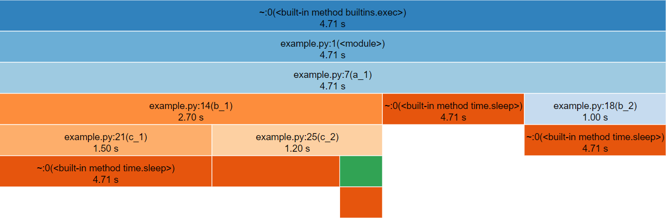
An icicle visualisation provided by snakeviz for the above Python code.

The third row represents a_1(), the only method called from global scope, therefore the first two rows represent Python’s internal code for launching our script and can be ignored (by clicking on the third row).

The row following a_1() is split into three boxes representing b_1(), time.sleep() and b_2(). Note that b_1() is called three times, but only has one box within the icicle diagram. The boxes are ordered left-to-right according to cumulative time, which happens to be the order they were first called.

If the box for time.sleep() is hovered it will change colour along with several other boxes that represent the other locations that time.sleep() was called from. Note that each of these boxes display the same duration, the timing statistics collected by cProfile (and visualised by snakeviz) are aggregate, so there is no information about individual method calls for methods which were called multiple times. This does however mean that if you check the properties to the left of the diagram whilst hovering time.sleep() you will see a cumulative time of 99% reported, the overhead of the method calls and for loop is insignificant in contrast to the time spent sleeping!

Below are the properties shown, the time may differ if you generated the profile yourself.

• Name: <built-in method time.sleep>
• Cumulative Time: 4.71 s (99.99 %)
• File: ~
• Line: 0
• Directory:

As time.sleep() is a core Python method it is displayed as “built-in method” and doesn’t have a file, line or directory.

If you hover any boxes representing the methods from the above code, you will see file and line properties completed. The directory property remains empty as the profiled code was in the root of the working directory. A profile of a large project with many files across multiple directories will see this filled.

Find the box representing c_2() on the icicle diagram, it’s children are unlabelled because they are not wide enough (but they can still be hovered). Clicking c_2() zooms in the diagram, showing the children to be time.sleep() and d_1().

To zoom back out you can either click the top row, which will zoom out one layer, or click “Reset Zoom” on the left-hand side.

In this simple example the execution is fairly evenly balanced between all of the user-defined methods, so there is not a clear hot-spot to investigate.

Below the icicle diagram, there is a table similar to the default output from cProfile. However, in this case you can sort the columns by clicking their headers and filter the rows shown by entering a filename in the search box. This allows built-in methods to be hidden, which can make it easier to highlight optimisation priorities.

Notebooks

If you followed along inside a notebook it might look like this:

The worked example inside a notebook.

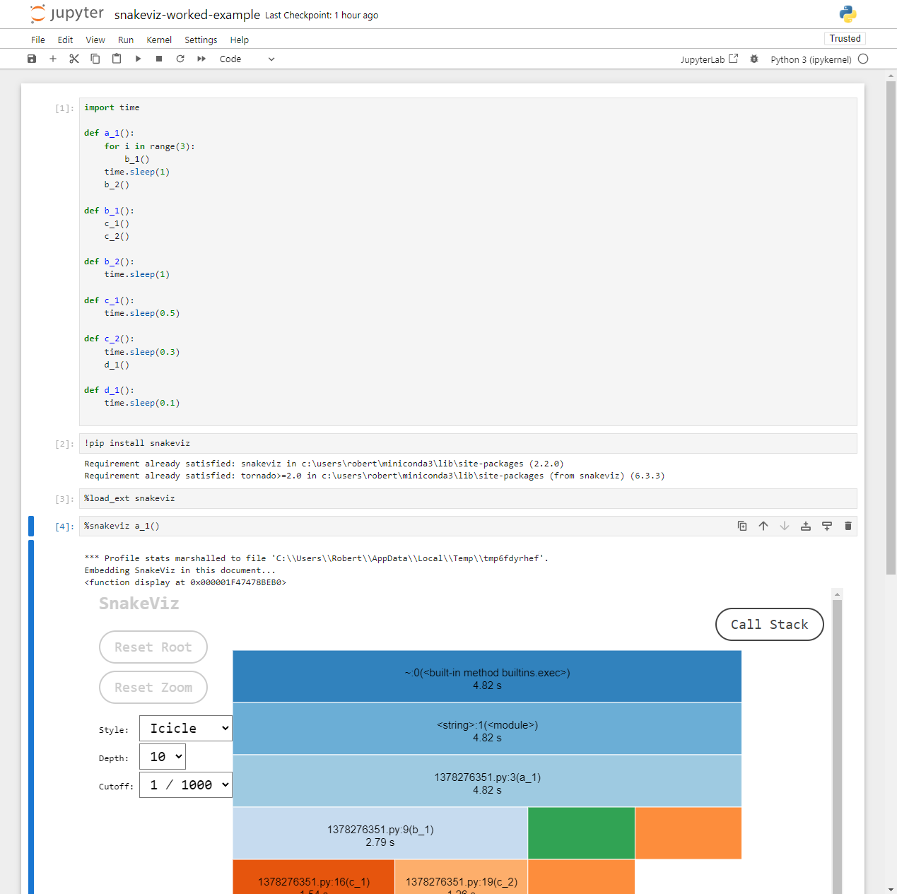
Because notebooks operate by creating temporary Python files, the filename (shown 1378276351.py above) and line numbers displayed are not too useful. However, the function names match those defined in the code and follow the temporary file name in parentheses, e.g. 1378276351.py:3(a_1), 1378276351.py:9(b_1) refer to the functions a_1() and b_1() respectively.

Sunburst

snakeviz provides an alternate “Sunburst” visualisation, accessed via the “Style” drop-down on the left-hand side.

This provides the same information as “Icicle”, however the rows are instead circular with the root method call found at the center.

The sunburst visualisation displays less text on the boxes, so it can be harder to interpret. However, it increases the visibility of boxes further from the root call.

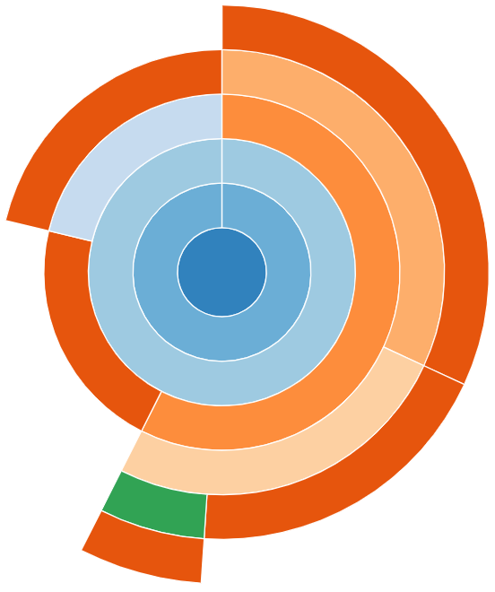
An sunburst visualisation provided by snakeviz for the worked example’s Python code.

Exercises

---

The following exercises allow you to review your understanding of what has been covered in this episode.

Exercise 1: Travelling Salesperson

Download and profile this Python program, try to locate the function call(s) where the majority of execution time is being spent.

The travelling salesperson problem aims to optimise the route for a scenario where a salesperson is requires to travel between N locations. They wish to travel to each location exactly once, in any order, whilst minimising the total distance travelled.

The provided implementation uses a naive brute-force approach.

The program can be executed via python travellingsales.py <cities>. The value of cities should be a positive integer, this algorithm has poor scaling so larger numbers take significantly longer to run.

Give me a hint

• If a hotspot isn’t visible with the argument 1, try increasing the value.
• If you think you identified the hotspot with your first profile, try investigating how the value of cities affects the hotspot within the profile.

Show me the solution

The hotspot only becomes visible when an argument of 5 or greater is passed.

You should see that distance() (from travellingsales.py:11) becomes the largest box (similarly it’s parent in the call-stack total_distance()) showing that it scales poorly with the number of cities. With 5 cities, distance() has a cumulative time of ~35% the runtime, this increases to ~60% with 9 cities.

Other boxes within the diagram correspond to the initialisation of imports, or initialisation of cities. These have constant or linear scaling, so their cost barely increases with the number of cities.

This highlights the need to profile a realistic test-case expensive enough that initialisation costs are not the most expensive component.

Exercise 2: Predator Prey

Download and profile the Python predator prey model, try to locate the function call(s) where the majority of execution time is being spent

This exercise uses the packages numpy and matplotlib, they can be installed via pip install numpy matplotlib.

The predator prey model is a simple agent-based model of population dynamics. Predators and prey co-exist in a common environment and compete over finite resources.

The three agents; predators, prey and grass exist in a two dimensional grid. Predators eat prey, prey eat grass. The size of each population changes over time. Depending on the parameters of the model, the populations may oscillate, grow or collapse due to the availability of their food source.

The program can be executed via python predprey.py.

It takes no arguments, but contains various environment properties which can be modified to change the model’s behaviour. When the model finishes it outputs a graph of the three populations predprey_out.png.

Show me the solution

It should be clear from the profile that the method Grass::eaten() (from predprey.py:278) occupies the majority of the runtime.

From the table below the Icicle diagram, we can see that it was called 1,250,000 times.

The top of the table shown by snakeviz.

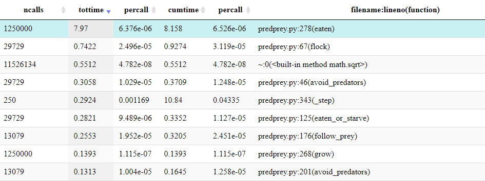
If the table is ordered by ncalls, it can be identified as the joint 4th most called method and 2nd most called method from predprey.py.

If you checked predprey_out.png (shown below), you should notice that there are significantly more Grass agents than Predators or Prey.

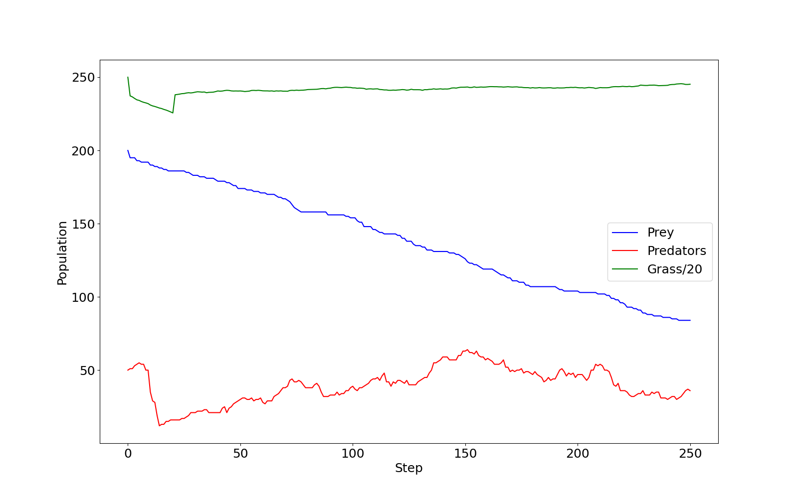
predprey_out.png as produced by the default configuration of predprey.py.

Similarly, the Grass::eaten() has a percall time is inline with other agent functions such as Prey::flock() (from predprey.py:67).

Maybe we could investigate this further with line profiling!

You may have noticed many iciles on the right hand of the diagram, these primarily correspond to the import of matplotlib which is relatively expensive!

Key Points

• A python program can be function level profiled with cProfile via python -m cProfile -o <output file> <script name> <arguments>.
• The output file from cProfile can be visualised with snakeviz via python -m snakeviz <output file>.
• Function level profiling output displays the nested call hierarchy, listing both the cumulative and total minus sub functions time.