Xarray is an extremely useful Python package for analysts working with N-Dimensional arrays, especially if they are stored as NetCDFs – the industry standard file structure for (e.g.) climate datasets.
The power of xarray comes from its ability to label N-Dimensional arrays, whereas the numpy and pandas packages can deal with unlabelled arrays (numpy) or labels in 2 dimensions only (pandas). Especially powerful is xarray’s ability to persist the labels however the arrays are sliced or chunked. The xarray syntax has been deliberately designed to be as similar as possible to pandas, which is familiar to many data scientists and generally considered to be very intuitive. The labels represent metadata and are structured into dimensions (e.g. time, latitude) and coordinate values (e.g. 24-09-2018, 67.064532) plus attributes.
The labelling enables operations on the data contained inside the xarray to be performed using the labels to specify axes for the operation or to isolate subsets of the data, just like in Pandas. It also means that users can use meaningful labels instead of axis numbers (e.g. axis=0) for operations, and there is no need to create dummy variables for aligning arrays like in numpy (np.newaxis). This makes operations over multiple arrays or array slices much easier to keep track of.
As well as sharing syntax, xarray is highly compatible with both pandas and numpy. Arrays can be swapped between numpy, pandas and xarray easily with xarray’s ncdata.to_array(), ncdata = xr.DataArray(array), ncdata.to_DataFrame() or ncdata = xr.Dataset(DataFrame) functions.
xarray also makes it easy to open, query, manipulate, concatenate, merge or visualise data stored in NetCDF files, or to save new data to NetCDF. NetCDFs are commonly used to store very large, labelled N-dimensional data; Xarray provides pandas-like syntax for handling them. Xarray avoids loading entire datasets into memory, instead it accesses data as and when it is needed meaning huge datasets can be loaded. An example is satellite imagery where labelled N-dimensional data for a given area may be repeated at many time points, all of which could be loaded, queried and manipulated using xarray.
Loading a NetCDF file is as simple as x = xr.open_dataset(netcdffile) and saving a dataframe or array to NetCDF is equally straighforward: DF.to_netCDF('filename').
Xarray is also tightly integrated with Dask so that operations over datasets too large to sit in memory can be achieved using Dask commands directly over xarray data arrays or datasets. Dask achieves this by chunking the dataset and distributing the computation over multiple cores. xarray takes a “chunks” argument that divides the xarray into dask arrays ready to be distributed. More information about xarray and dask is avilable in the (very good) documentation.
xarray works with two basic data structures – the DataArray and the DataSet.
A DataArray is a labelled N-dimensional array - this can come from a pandas dataframe with labels or N-dimensional unlabelled numpy arrays. Metadata and attributes can then be added.
A DataSet is a collection of DataArrays. The power of the Dataset structure comes from the ability to perform operations over multiple arrays along shared dimensions.
In this example I use xarray to load in a dataset from a NetCDF file. The dataset includes layers representing 2D maps of a section of the Greenland Ice Sheet imaged using the ESA satellite Sentinel-2. Sentinel-2 images the surface in nine wavelengths (‘bands) at 20m ground resolution so there are actually nine layers for each image, each one projected identically in space (there was some preprocessing of these data using GDAL that I will not cover here). The layers are loaded in using xarray, converted to numpy arrays and processed, then saved to a new NetCDF with metadata and attributes. xarray’s plot function is used to display the key layers.
First the necessary packages are imported and the image bands are loaded in from a NetCDF file using xarray. Only the reflectance values are extracted from the data array and saved to a 9D numpy array, where each dimension represents a wavelength.
import xarray as xr
import numpy as np
import matplotlib.pyplot as plt
from sklearn.externals import joblib

S2vals = np.zeros([9,5490,5490]) #set up array
bands = ['02','03','04','05','05','07','08','11','12'] # Band numbers
for i in np.arange(0,len(bands),1): #loop through bands in NetCDF file
    S2BX = xr.open_dataset(str(img_path+'B'+bands[i]+'.nc')) # open only the relevant band from the NetCDF
    S2BXarr = S2BX.to_array() # send the band to a numpy array
    S2BXvals = np.array(S2BXarr.variable.values[1]) # extract only the reflectance values
    S2BXvals = S2BXvals.astype(float) #convert to float
    S2vals[i,:,:] = S2BXvals # append to 'master' ND array
S2vals = vals/10000 # correct unit from S2 L2A data to reflectance between 0-1
In the next stage, a scikit-learn classifier is applied to the 9D array. This classifier has been trained in a separate script, saved to a .pkl file and then loaded in here. The 9D array is also converted into a layer that applies a conversion formula to predict the albedo -or reflectivity - of the surface. This is a stripped down version of the code developed in my IceSurfClassifiers GitHub repository - go there for the complete scripts.
#load pickled model
clf = joblib.load('/home/Code/Sentinel2_classifier.pkl')

    # get dimensions of each band layer
    lenx, leny = np.shape(S2vals[0])

    # convert image bands into single 9-dimensional numpy array
    S2valsT = S2vals.reshape(9, lenx * leny)  # reshape into 5 x 1D arrays
    S2valsT = S2valsT.transpose()  # transpose so that bands are read as features


    # create albedo array by applying Knap (1999) narrowband - broadband conversion
    albedo_array = np.array([0.356 * (S2vals[0]) + 0.13 * (S2vals[2]) + 0.373 * (
            S2vals[6]) + 0.085 * (S2vals[7]) + 0.072 * (S2vals[8]) - 0.0018])

    # apply classifier to each pixel - predict surface type
    predicted = clf.predict(S2valsT)
    predicted = np.array(predicted)

    # convert surface class (string) to a numeric value for plotting
    predicted[predicted == 'SN'] = float(1)
    predicted[predicted == 'WAT'] = float(2)
    predicted[predicted == 'CC'] = float(3)
    predicted[predicted == 'CI'] = float(4)
    predicted[predicted == 'LA'] = float(5)
    predicted[predicted == 'HA'] = float(6)
    predicted[predicted == 'Zero'] = float(0)

    # reshape 1D array back into original image dimensions
    predicted = np.reshape(predicted, [lenx, leny])
    albedo = np.reshape(albedo_array, [lenx, leny])
There is now a classified surface map and an albedo map in memory. The next section shows how this is collated into an xarray dataset with some metadata and saved to a new NetCDF file.
    # add predicted map array and add metadata
    # note that coords_geo are obtained from the original projection info and extracted using gdal - not shown here.
    predictedxr = xr.DataArray(predicted, coords=coords_geo, dims=['y', 'x'])
    predictedxr.name = 'Surface Class'
    predictedxr.attrs['long_name'] = 'Surface classified using Random Forest'
    predictedxr.attrs['units'] = 'None'

    # add albedo map array and add metadata
    albedoxr = xr.DataArray(albedo, coords=coords_geo, dims=['y', 'x'])
    albedoxr.name = 'Surface albedo computed after Knap et al. (1999) narrowband-to-broadband conversion'
    albedoxr.attrs['units'] = 'dimensionless'

    # collate data arrays into a dataset
    dataset = xr.Dataset({
        'classified': (['x', 'y'], predictedxr),
        'albedo': (['x', 'y'], albedoxr),
    })

    # add some high-level metadata for dataset
    dataset.attrs[
        'title'] = 'Classified surface and albedo maps produced from Sentinel-2 ' \
                   'imagery of the Greenland Ice Sheet: {}'.format(area_label)

    # save dataset to netcdf
    dataset.to_netcdf(savefig_path + "Classification_and_Albedo_Data_{}.nc".format(area_label))
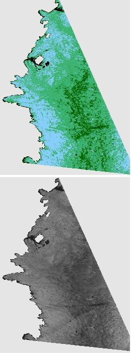
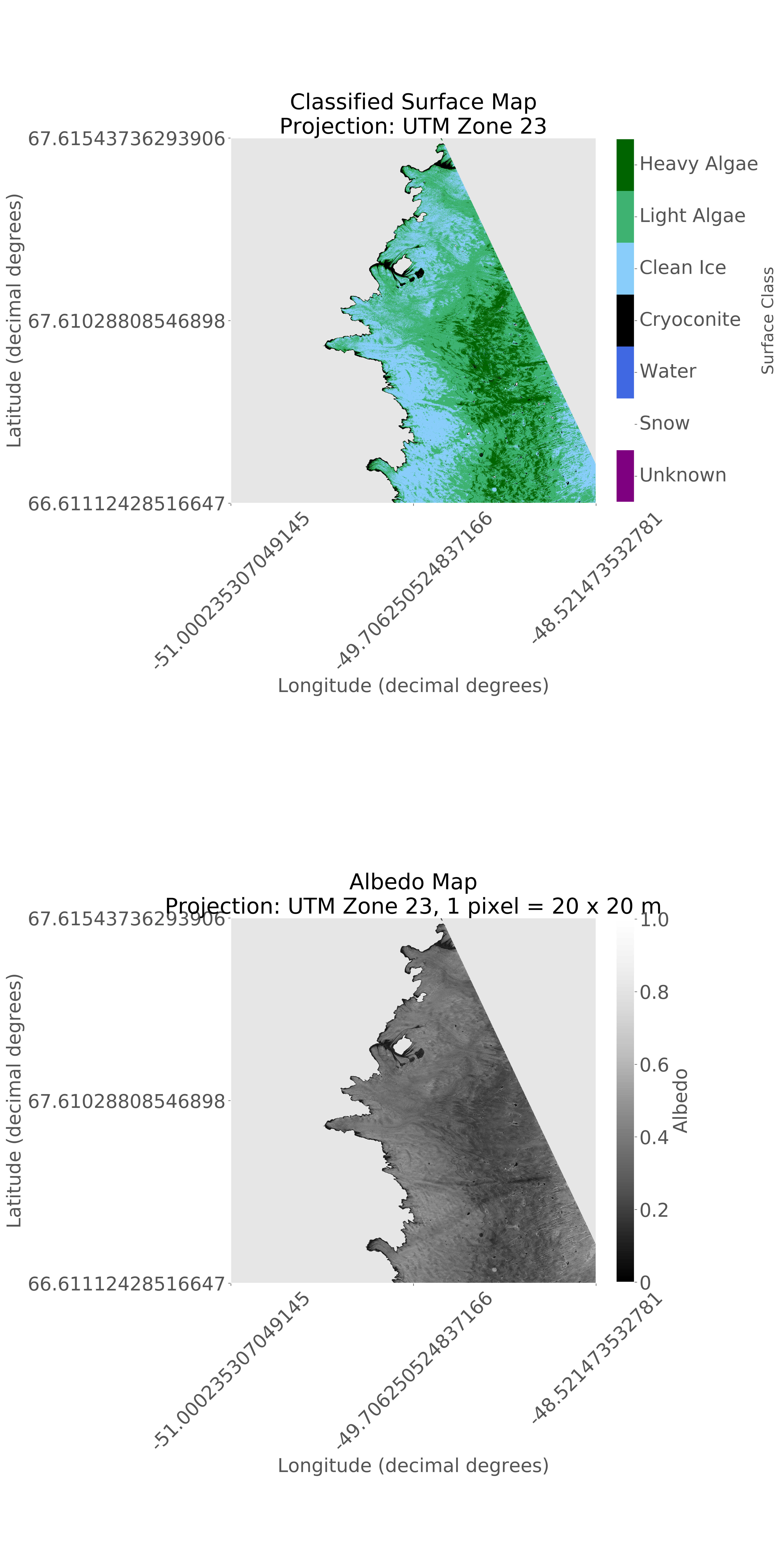
xarrays plot function (built on matplotlib) can then be used to visualise the layers (classified surface above, albedo map below).
dataset.classified.plot()
dataset.albedo.plot()

Note that in reality there was some more formatting applied prior to plotting, including masking out non-ice areas and georeferencing. The xarray plot function is built on matplotib so the syntax for formatting plots is consistent, and labels, ticks, titles, colorbars etc ca easily be added. Here is a decorated version using matplotlib commands to the xarray plot:

xarray is a powerful tool for working with large structured, labelled datasets. It is quite intuitive to users familiar with numpy and pandas and plays well with both. It also provides a neat route to standardised data archiving in NetCDF format with metadata and attributes stored alongside the data.
More info about xarray is available in the documentation and several excellent blogs. The code shown above is a reduced version from this repository.
For queries relating to collaborating with the RSE team on projects: rse@sheffield.ac.uk
Information and access to Bede.
Join our mailing list so as to be notified when we advertise talks and workshops by subscribing to this Google Group.
Queries regarding free research computing support/guidance should be raised via our Code clinic or directed to the University IT helpdesk.
List of archived pages: Archive.