Data visualisation in C++ with computational models

A guest post by Seb James, Research Associate, Department of Psychology (GitHub; Twitter).

---

In this blog post I’m going to talk about data visualisation - making graphs - within C++ programs. I’ll describe why you might want to do this and I’ll try to justify why I’ve spent a sizeable part of my time over the last couple of years developing graphing code in C++, rather than using Python or R like everyone else! The code I’ll discuss is available at https://github.com/ABRG-Models/morphologica.

Most of the academic blog posts and videos about data visualisation that I see refer to scripted languages like Python, R or MATLAB. These languages have the ability to render high quality graphs and they provide convenient function calls to create standard graphs such as scatter plots and bar graphs, as well as more esoteric visualisations such as Sankey plots or Dendrograms (see the d3 graph gallery for lots of interesting examples). It’s easy to generate output in a standard format like PNG or PDF and so if you’re visualising an existing dataset then one of these scripted languages – Python with matplotlib or R with ggplot2 – is probably the best way to communicate information about the data to your audience.

Scripted languages have become the richest platforms for data visualisation because they are so convenient and flexible. There is no need to compile your program or concern yourself with the complexities of linking libraries; you just write the script in a text editor and execute it with the interpreter. The script can be easily archived, making your work more reproducible and it is straightforward to apply a given data visualisation routine to many different datasets. For these reasons, scripted data visualisations are more popular in the academic community than visualisation using a dedicated graphing application.

Although interpreted programs are always slower than compiled code, with today’s average laptop or PC the compute time required to draw most graphs is minimal and so there is no incentive to use a faster, compiled language such as C++ with its additional development overhead (more lines of code for headers, a need to compile before running, the need to specify library links).

So why this post about data visualisation in C++? While the wider data-vis community won’t see C++ as a primary tool, there is a use case for researchers who write numerically intensive models - any model which ‘contains’ a lot of numbers and benefits from making maximal use of available computational resources. My work falls into this category. Although I don’t need racks of servers to run my 2D reaction-diffusion models, each simulation takes a minute or two to run, making use of multiple CPU cores. On past experience, I’d expect these programs to run about an order of magnitude slower in Python or MATLAB. In practice, rather than waiting longer, I would limit the resolution, or scope of the model to keep the time it required to run at an optimum value. A batch of simulations running overnight is much more useful than a batch which needs a week to complete. However, by limiting the scope of the model, I might be ignoring science that would only present itself in a higher resolution system. Put simply, using C++ allows me to get the most out of the computer hardware I have access to.

Even if there’s a clear case for using compiled code to simulate, it’s not a given that the data should be visualised this way. A common approach is to have the compiled program write data into a file (plug: I use morph::HdfData to write HDF5 files), and then use Python or R to construct the graphs. This is perfectly sensible for generating graphs for a journal or report, but it can be clunky when visualising to inspect the model. Model inspection is a manual exploration of the model, watching its behaviour for hand-selected parameter choices. This process of manual exploration is part of the development of every model. First, it’s essential to verify that the code works as expected and that it expresses the mathematics of the model correctly. The ability to graph the state of the internal variables of the model, possibly from one timestep to the next, is exceedingly helpful as part of the debugging process. Once the model is generating believable output, manual exploration can aid the researcher in determining suitable parameter ranges over which the model is stable. I find this important for planning batched parameter searches or parameter optimisations. If the model is dynamic, it is also very helpful to see the dynamics unfold in real-time and to have the ability to create movies of the simulation. For these reasons, I consider it a necessity to be able to visualise data in C++ simulations.

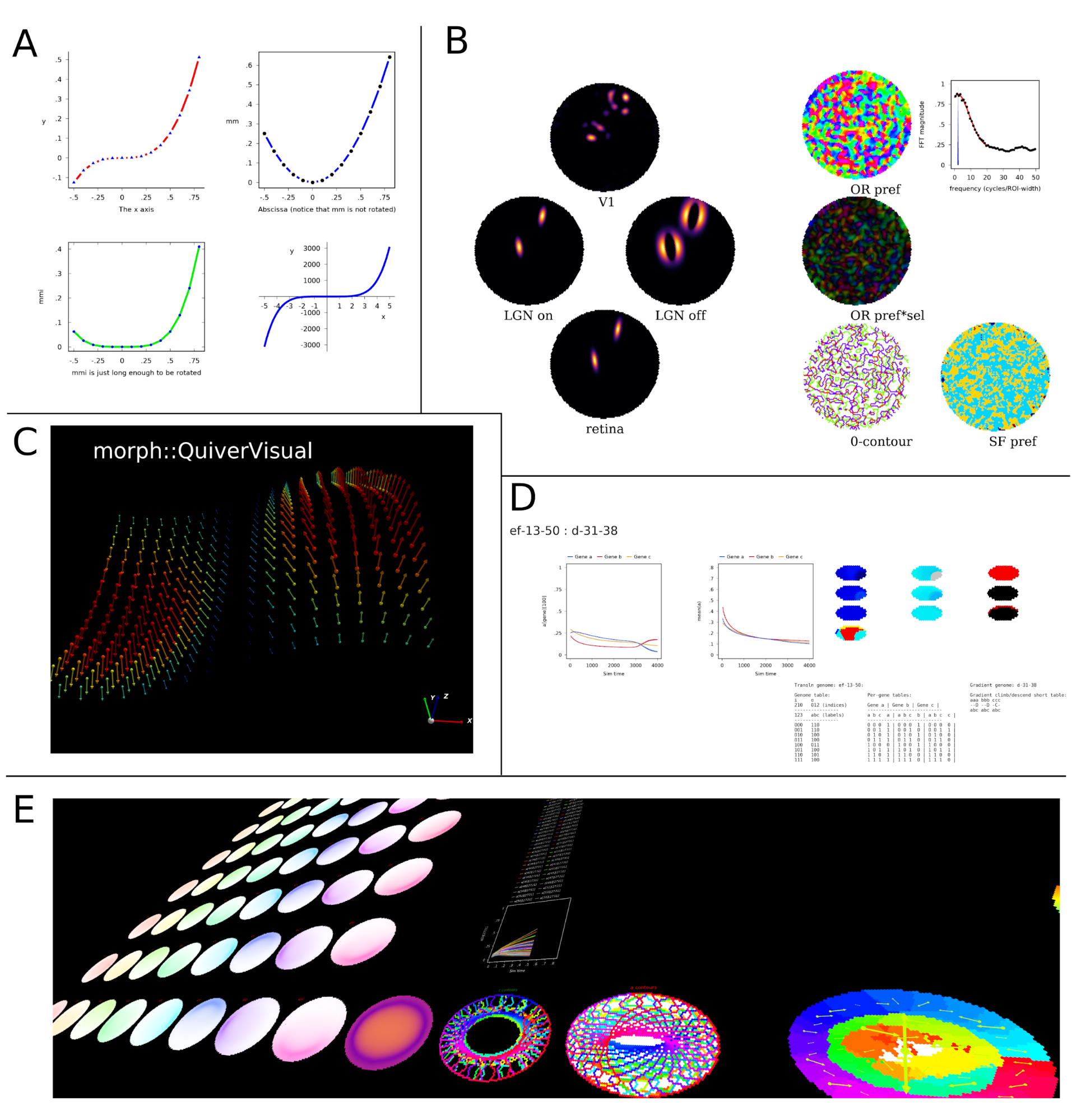
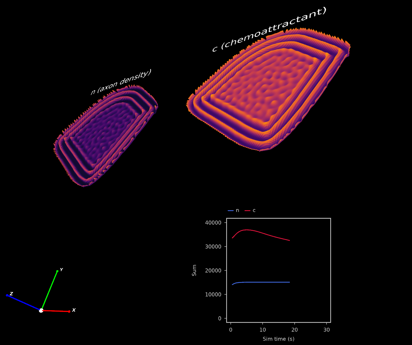
Unfortunately, there’s no natural choice of library for graphing with C++; nothing quite as ubiquitous as matplotlib for Python. matplot++ is probably the most mature graphing library for C++, though it appears to be somewhat of a clone of matplotlib, intended for drawing static graphs for publication, and I find it hard to see why you wouldn’t just graph with matplotlib itself, for convenience. In my work, during the debugging process I may need visualisations of three-dimensional surfaces in models with as many as 100 state variables. In other words, to watch the full model may involve plotting a hundred 3D graphs at once! Not only do I need to visualise my data, I need to do so with minimal use of the processor. This need for efficient data visualisation motivated me to develop the from-scratch graphing code found in morphologica.

To write the code, I was inspired by gaming technology. My kids play a game called Garry’s Mod. Garry’s Mod isn’t actually a game at all, it’s a physics sandbox; a 3D environment into which you can place models with which you can interact. Really, it’s an example of a game engine. I imagined building a similar world into which I could place graph models which would update as my simulations progressed. I wanted to fly around the graphs, viewing them from any angle and bringing as many into the view as necessary. A lot of the work rendering the scene would be carried out on my graphics processor, leaving my CPU free to compute the model. The output of the visualisation, which could be captured as screenshots, wouldn’t necessarily need to be of publication quality - a traditional approach using Python and matplotlib could be used to generate additional analysis and final graphs for a paper.

For this ‘game engine for visualisation’, I chose the name morph::Visual. The code would form part of morphologica, a collection of simulation support facilities whose namespace name is morph (morphologica suggests simulations relating to morphology, a theme in our group). I chose to use modern OpenGL to program the graphics, because it is cross-platform, well established and efficient. The modern in the name indicates that a special shader program, which runs on the GPU, must be written to update the view of the scene. In OpenGL, everything is drawn as triangles. A line is two long, thin triangles. A sphere is a grid of triangles; mine have a fan at the top of the sphere, then rings from the top to the bottom, with a final fan finishing the sphere off, which seemed easier than making a truncated icosahedron! It’s a very low-level approach to graphics, and no small task to develop from scratch, but initially, all I needed was surfaces made up of hexagons, which are easily constructed from triangles.

I chose an architecture in which each graph visualisation was a class derived from a base class called morph::VisualModel. The first VisualModels were HexGridVisual and CoordArrows; these were the only objects in my first scenes. Later, I added other VisualModels, including morph::GraphVisual, which makes it easy to create a regular 2D line or scatter graph. This has given me the opportunity to try to develop a more intuitive API than the one provided by matplotlib in Python (and copied in matplot++), which I have always found confusing (there always seem to be too many ways to achieve a result). In morph::Visual, I can make decisions about how I think the API should work and I can favour simplicity over flexibility.

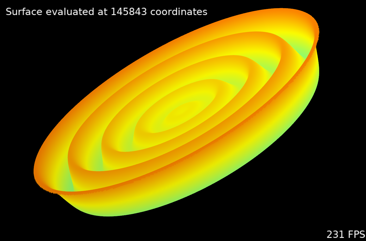
The results have been very satisfying. I am able to run huge visualisations with more than 50 3D graphs. A surface plot containing 145000 coordinates can be updated and visualised at 4K screen resolution in as little as 4.3 milliseconds of compute time (see the morphologica examples/fps.cpp). The API to create a graph object and then update the data being displayed is straightforward to use. Anyone using the code gets all the ‘hard stuff’ for free - projecting the data, reverse projecting mouse movements to give an intuitive user interface, lighting effects in the shader, nice colour maps and the ability to use TrueType text (which is a big faff in OpenGL!) are all handled for you. The code is header-only, and the TrueType fonts used for text rendering are all compiled into your binaries, avoiding annoying ‘resource not available’ runtime messages.

morphologica is in use across our research group, but it is emphatically not intended to be limited to any particular field of research and we’d love to see others making use of it. You’ll find that it’s a useful library of ‘simulation support facilities’ and I warmly invite you to try it out in your own C++ simulation code.

---

This post was also published on the University of Sheffield Data Visualisation hub, which features information, tutorials and a showcase of many aspects of data visualisation.