

All in One View
Content from Introduction to Profiling
Last updated on 2025-03-24 | Edit this page
Estimated time: 25 minutes
Overview
Questions
- Why should you profile your code?
- How should you choose which type of profiler to use?
- Which test case should be profiled?
Objectives
- explain the benefits of profiling code and different types of profiler
- identify the appropriate Python profiler for a given scenario
- explain how to select an appropriate test case for profiling and why
Introduction
Performance profiling is the process of analysing and measuring the performance of a program or script, to understand where time is being spent during execution.
Profiling is useful when you have written any code that will be running for a substantial period of time. As your code grows in complexity, it becomes increasingly difficult to estimate where time is being spent during execution. Profiling allows you to narrow down where the time is being spent, to identify whether this is of concern or not.
Profiling is a relatively quick process which can either provide you the peace of mind that your code is efficient, or highlight the performance bottleneck. There is limited benefit to optimising components that may only contribute a tiny proportion of the overall runtime. Identifying bottlenecks allows optimisation to be precise and efficient, potentially leading to significant speedups enabling faster research. In extreme cases, addressing bottlenecks has enabled programs to run hundreds or thousands of times faster!
Increasingly, particularly with relation to HPC, attention is being paid to the energy usage of software. Profiling your software will provide you the confidence that your software is an efficient use of resources.
When to Profile
Profiling is most relevant to working code, when you have reached a stage that the code works and are considering deploying it.
Any code that will run for more than a few minutes over its lifetime and isn’t a quick one-off script can benefit from profiling.
Profiling should be a relatively quick and inexpensive process. If there are no significant bottlenecks in your code you can quickly be confident that your code is reasonably optimised. If you do identify a concerning bottleneck, further work to optimise your code and reduce the bottleneck could see significant improvements to the performance of your code and hence productivity.
All Programmers Can Benefit
Even professional programmers make oversights that can lead to poor performance, and can be identified through profiling.
For example Grand Theft Auto Online, which has allegedly earned over $7bn since it’s 2013 release, was notorious for it’s slow loading times. 8 years after it’s release a ‘hacker’ had enough, they reverse engineered and profiled the code to enable a 70% speedup!
How much revenue did that unnecessary bottleneck cost, through user churn?
How much time and energy was wasted, by unnecessarily slow loading screens?
The bottlenecked implementation was naively parsing a 10MB JSON file to create a list of unique items.
Repeatedly:
- Checking the length of (C) strings, e.g. iterating till the terminating character is found, resolved by caching the results.
- Performing a linear search of a list to check for duplicates before
inserting, resolved by using an appropriate data structure (dictionary).
- Allegedly duplicates were never even present in the JSON.
Why wasn’t this caught by one of the hundreds of developers with access to the source code?
Was more money saved by not investigating performance than committing time to profiling and fixing the issue?
Types of Profiler
There are multiple approaches to profiling, most programming languages have one or more tools available covering these approaches. Whilst these tools differ, their core functionality can be grouped into several categories.
Manual Profiling
Similar to using print() for debugging, manually timing
sections of code can provide a rudimentary form of profiling.
PYTHON
import time

t_a = time.monotonic()
# A: Do something
t_b = time.monotonic()
# B: Do something else
t_c = time.monotonic()
# C: Do another thing
t_d = time.monotonic()

mainTimer_stop = time.monotonic()
print(f"A: {t_b - t_a} seconds")
print(f"B: {t_c - t_b} seconds")
print(f"C: {t_d - t_c} seconds")
Above is only one example of how you could manually profile your Python code, there are many similar techniques.
Whilst this can be appropriate for profiling narrow sections of code, it becomes increasingly impractical as a project grows in size and complexity. Furthermore, it’s also unproductive to be routinely adding and removing these small changes if they interfere with the required outputs of a project.
Benchmarking
You may have previously used timeit
for timing Python code.
This package returns the total runtime of an isolated block of code, without providing a more granular timing breakdown. Therefore, it is better described as a tool for benchmarking.
Function-Level Profiling
Software is typically comprised of a hierarchy of function calls, both functions written by the developer and those used from the language’s standard library and third party packages.
Function-level profiling analyses where time is being spent with respect to functions. Typically, function-level profiling will calculate the number of times each function is called and the total time spent executing each function, inclusive and exclusive of child function calls.
This allows functions that occupy a disproportionate amount of the total runtime to be quickly identified and investigated.
In this course we will cover the usage of the function-level profiler
cProfile and how it’s output can be visualised with
snakeviz.
Line-Level Profiling
Function-level profiling may not always be granular enough, perhaps your software is a single long script, or function-level profiling highlighted a particularly complex function.
Line-level profiling provides greater granularity, analysing where time is being spent with respect to individual lines of code.
This will identify individual lines of code that occupy an disproportionate amount of the total runtime.
In this course we will cover the usage of the line-level profiler
line_profiler.
Deterministic vs Sampling Profilers
Line-level profiling can be particularly expensive, a program can execute hundreds of thousands of lines of code per second. Therefore, collecting information about each line of code can be costly.
line_profiler is deterministic, meaning that it tracks
every line of code executed. To avoid it being too costly, the profiling
is restricted to methods targeted with the decorator
@profile.
In contrast, scalene
is a more advanced Python profiler capable of line-level profiling. It
uses a sampling based approach, whereby the profiler halts and samples
the line of code currently executing thousands of times per second. This
reduces the cost of profiling, whilst still maintaining representative
metrics for the most expensive components.
Timeline Profiling
Timeline profiling takes a different approach to visualising where time is being spent during execution.
Typically, a subset of function-level profiling, the execution of the profiled software is instead presented as a timeline highlighting the order of function execution in addition to the time spent in each individual function call.
By highlighting individual functions calls, patterns relating to how performance scales over time can be identified. These would be hidden with the aforementioned aggregate approaches.
viztracer
is an example of a timeline profiler for Python, however we won’t be
demonstrating timeline profiling on this course.
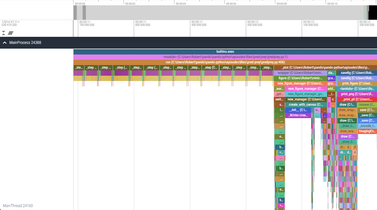
viztracer/vizviewer.Hardware Metric Profiling
Processor manufacturers typically release advanced profilers specific to their hardware with access to internal hardware metrics. These profilers can provide analysis of performance relative to theoretical hardware maximums (e.g. memory bandwidth or operations per second) and detail the utilisation of specific hardware features and operations.
Using these advanced profilers requires a thorough understanding of the relevant processor architecture and may lead to hardware specific optimisations.
Examples of these profilers include; Intel’s VTune, AMD’s uProf, and NVIDIA’s Nsight Compute.
Profiling of this nature is outside the scope of this course.
Selecting an Appropriate Test Case
The act of profiling your code, collecting additional timing metrics during execution, will cause your program to execute slower. The slowdown is dependent on many variables related to both your code and the granularity of metrics being collected.
Similarly, the longer your code runs, the more code that is being executed, the more data that will be collected. A profile that runs for hours could produce gigabytes of output data!
Therefore, it is important to select an appropriate test-case that is both representative of a typical workload and small enough that it can be quickly iterated. Ideally, it should take no more than a few minutes to run the profiled test-case from start to finish, however you may have circumstances where something that short is not possible.
For example, you may have a model which normally simulates a year in hourly time-steps. It would be appropriate to begin by profiling the simulation of a single day. If the model scales over time, such as due to population growth, it may be pertinent to profile a single day later into a simulation if the model can be resumed or configured. A larger population is likely to amplify any bottlenecks that scale with the population, making them easier to identify.
Exercise (5 minutes)
Think about a project where you’ve been working with Python. Do you know where the time during execution is being spent?
Write a short plan of the approach you would take to investigate and confirm where the majority of time is being spent during its execution.
- What tools and techniques would be required?
- Is there a clear priority to these approaches?
- Which test-case/s would be appropriate?
- Profiling is a relatively quick process to analyse where time is being spent and bottlenecks during a program’s execution.
- Code should be profiled when ready for deployment if it will be running for more than a few minutes during its lifetime.
- There are several types of profiler each with slightly different
purposes.
- function-level:
cProfile(visualised withsnakeviz) - line-level:
line_profiler - timeline:
viztracer - hardware-metric
- function-level:
- A representative test-case should be profiled, that is large enough to amplify any bottlenecks whilst executing to completion quickly.
Content from Function Level Profiling
Last updated on 2025-05-11 | Edit this page
Estimated time: 40 minutes
Overview
Questions
- When is function level profiling appropriate?
- How can
cProfileandsnakevizbe used to profile a Python program? - How are the outputs from function level profiling interpreted?
Objectives
- execute a Python program via
cProfileto collect profiling information about a Python program’s execution - use
snakevizto visualise profiling information output bycProfile - interpret
snakevizviews, to identify the functions where time is being spent during a program’s execution
Introduction
Software is typically comprised of a hierarchy of function calls, both functions written by the developer and those used from the language’s standard library and third party packages.
Function-level profiling analyses where time is being spent with respect to functions. Typically function-level profiling will calculate the number of times each function is called and the total time spent executing each function, inclusive and exclusive of child function calls.
This allows functions that occupy a disproportionate amount of the total runtime to be quickly identified and investigated.
In this episode we will cover the usage of the function-level
profiler cProfile, how it’s output can be visualised with
snakeviz and how the output can be interpreted.
What is a Call Stack?
The call stack keeps track of the active hierarchy of function calls and their associated variables.
As a stack it is a last-in first-out (LIFO) data structure.
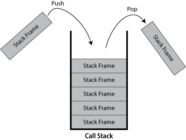
When a function is called, a frame to track its variables and metadata is pushed to the call stack. When that same function finishes and returns, it is popped from the stack and variables local to the function are dropped.
If you’ve ever seen a stack overflow error, this refers to the call stack becoming too large. These are typically caused by recursive algorithms, whereby a function calls itself, that don’t exit early enough.
Within Python the current call-stack can be printed using the core
traceback package, traceback.print_stack()
will print the current call stack.
The below example:
PYTHON
import traceback

def a():
    b1()
    b2()
def b1():
    pass
def b2():
    c()
def c():
    traceback.print_stack()

a()
Here we can see that the printing of the stack trace is called in
c(), which is called by b2(), which is called
by a(), which is called from global scope.
Hence, this prints the following call stack:
OUTPUT
  File "C:\call_stack.py", line 13, in <module>
    a()
  File "C:\call_stack.py", line 5, in a
    b2()
  File "C:\call_stack.py", line 9, in b2
    c()
  File "C:\call_stack.py", line 11, in c
    traceback.print_stack()
The first line states the file and line number where a()
was called from (the last line of code in the file shown). The second
line states that it was the function a() that was called,
this could include its arguments. The third line then repeats this
pattern, stating the line number where b2() was called
inside a(). This continues until the call to
traceback.print_stack() is reached.
You may see stack traces like this when an unhandled exception is thrown by your code.
In this instance the base of the stack has been printed first, other visualisations of call stacks may use the reverse ordering.
cProfile
cProfile
is a function-level profiler provided as part of the Python standard
library.
It can be called directly within your Python code as an imported package, however it’s easier to use its script interface:
For example if you normally run your program as:
You would call cProfile to produce profiling output
out.prof with:
No additional changes to your code are required, it’s really that simple!
If you instead, don’t specify output to file (e.g. remove
-o out.prof from the command), cProfile will
produce output to console similar to that shown below:
OUTPUT
         28 function calls in 4.754 seconds

   Ordered by: standard name

   ncalls  tottime  percall  cumtime  percall filename:lineno(function)
        1    0.000    0.000    4.754    4.754 worked_example.py:1(<module>)
        1    0.000    0.000    1.001    1.001 worked_example.py:13(b_2)
        3    0.000    0.000    1.513    0.504 worked_example.py:16(c_1)
        3    0.000    0.000    1.238    0.413 worked_example.py:19(c_2)
        3    0.000    0.000    0.334    0.111 worked_example.py:23(d_1)
        1    0.000    0.000    4.754    4.754 worked_example.py:3(a_1)
        3    0.000    0.000    2.751    0.917 worked_example.py:9(b_1)
        1    0.000    0.000    4.754    4.754 {built-in method builtins.exec}
       11    4.753    0.432    4.753    0.432 {built-in method time.sleep}
        1    0.000    0.000    0.000    0.000 {method 'disable' of '_lsprof.Profiler' objects}
The columns have the following definitions:
| Column | Definition |
|---|---|
ncalls |
The number of times the given function was called. |
tottime |
The total time spent in the given function, excluding child function calls. |
percall |
The average tottime per function call
(tottime/ncalls). |
cumtime |
The total time spent in the given function, including child function calls. |
percall |
The average cumtime per function call
(cumtime/ncalls). |
filename:lineno(function) |
The location of the given function’s definition and it’s name. |
This output can often exceed the terminal’s buffer length for large
programs and can be unwieldy to parse, so the package
snakeviz is often utilised to provide an interactive
visualisation of the data when exported to file.
snakeviz
It can help to run these examples by running snakeviz
live. For the worked example you may wish to also show the code (e.g. in
split screen).
Demonstrate features such as moving up/down the call-stack by clicking the boxes and changing the depth and cutoff via the dropdown.
Download pre-generated profile reports:
snakeviz example screenshot: files/schelling_out.prof
Worked example: files/snakeviz-worked-example/out.prof
snakeviz
is a web browser based graphical viewer for cProfile output
files.
It is not part of the Python standard library, and therefore must be
installed via pip.
Once installed, you can visualise a cProfile output file
such as out.prof via:
This should open your web browser displaying a page similar to that below.
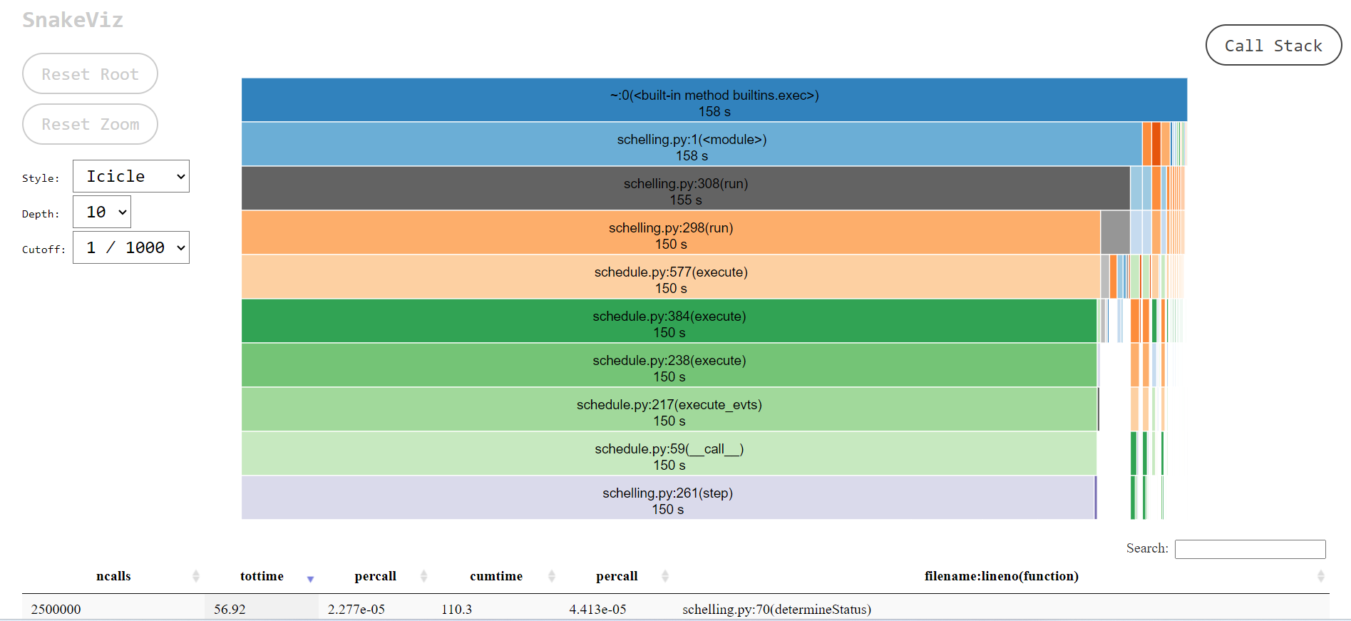
snakeviz.The icicle diagram displayed by snakeviz represents an
aggregate of the call stack during the execution of the profiled code.
The box which fills the top row represents the root call, filling the
row shows that it occupied 100% of the runtime. The second row holds the
child methods called from the root, with their widths relative to the
proportion of runtime they occupied. This continues with each subsequent
row, however where a method only occupies 50% of the runtime, its
children can only occupy a maximum of that runtime hence the appearance
of “icicles” as each row gets narrower when the overhead of methods with
no further children is accounted for.
By clicking a box within the diagram, it will “zoom” making the selected box the root allowing more detail to be explored. The diagram is limited to 10 rows by default (“Depth”) and methods with a relatively small proportion of the runtime are hidden (“Cutoff”).
As you hover each box, information to the left of the diagram updates specifying the location of the method and for how long it ran.
snakeviz Inside Notebooks
If you’re more familiar with writing Python inside Jupyter notebooks
you can still use snakeviz directly from inside notebooks
using the notebooks “magic” prefix (%) and it will
automatically call cProfile for you.
First snakeviz must be installed and its extension
loaded.
Following this, you can either call %snakeviz to profile
a function defined earlier in the notebook.
Or, you can create a %%snakeviz cell, to profile the
python executed within it.
In both cases, the full snakeviz profile visualisation
will appear as an output within the notebook!
You may wish to right click the top of the output, and select “Disable Scrolling for Outputs” to expand its box if it begins too small.
Worked Example
Demonstrate this!
To more clearly demonstrate how an execution hierarchy maps to the icicle diagram, the below toy example Python script has been implemented.
PYTHON
import time

def a_1():
    for i in range(3):
        b_1()
    time.sleep(1)
    b_2()

def b_1():
    c_1()
    c_2()

def b_2():
    time.sleep(1)

def c_1():
    time.sleep(0.5)

def c_2():
    time.sleep(0.3)
    d_1()

def d_1():
    time.sleep(0.1)

# Entry Point
a_1()
All of the methods except for b_1() call
time.sleep(), this is used to provide synthetic bottlenecks
to create an interesting profile.
-
a_1()callsb_1()x3 andb_2()x1 -
b_1()callsc_1()x1 andc_2()x1 -
c_2()callsd_1()
Follow Along
Download the
Python
source for the example or
cProfile
output file and follow along with the worked example on your own
machine.
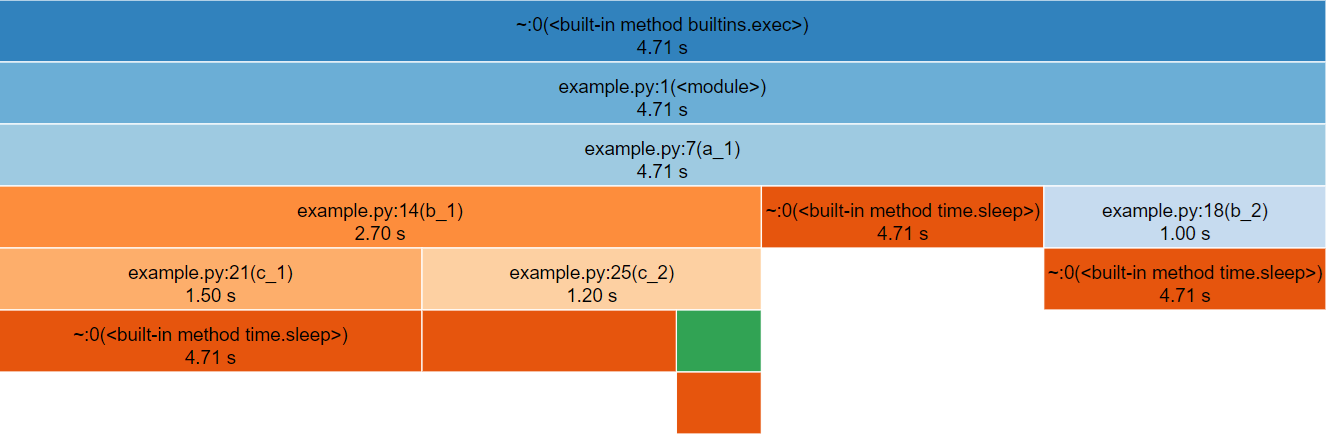
snakeviz for the above Python code.The third row represents a_1(), the only method called
from global scope, therefore the first two rows represent Python’s
internal code for launching our script and can be ignored (by clicking
on the third row).
The row following a_1() is split into three boxes
representing b_1(), time.sleep() and
b_2(). Note that b_1() is called three times,
but only has one box within the icicle diagram. The boxes are ordered
left-to-right according to cumulative time, which happens to be the
order they were first called.
If the box for time.sleep() is hovered it will change
colour along with several other boxes that represent the other locations
that time.sleep() was called from. Note that each of these
boxes display the same duration, the timing statistics collected by
cProfile (and visualised by snakeviz) are
aggregate, so there is no information about individual method calls for
methods which were called multiple times. This does however mean that if
you check the properties to the left of the diagram whilst hovering
time.sleep() you will see a cumulative time of 99%
reported, the overhead of the method calls and for loop is insignificant
in contrast to the time spent sleeping!
Below are the properties shown, the time may differ if you generated the profile yourself.
-
Name:
<built-in method time.sleep> -
Cumulative Time:
4.71 s (99.99 %) -
File:
~ -
Line:
0 - Directory:
As time.sleep() is a core Python method it is displayed
as “built-in method” and doesn’t have a file, line or directory.
If you hover any boxes representing the methods from the above code, you will see file and line properties completed. The directory property remains empty as the profiled code was in the root of the working directory. A profile of a large project with many files across multiple directories will see this filled.
Find the box representing c_2() on the icicle diagram,
its children are unlabelled because they are not wide enough (but they
can still be hovered). Clicking c_2() zooms in the diagram,
showing the children to be time.sleep() and
d_1().
To zoom back out you can either click the top row, which will zoom out one layer, or click “Reset Zoom” on the left-hand side.
In this simple example the execution is fairly evenly balanced between all of the user-defined methods, so there is not a clear hot-spot to investigate.
Below the icicle diagram, there is a table similar to the default
output from cProfile. However, in this case you can sort
the columns by clicking their headers and filter the rows shown by
entering a filename in the search box. This allows built-in methods to
be hidden, which can make it easier to highlight optimisation
priorities.
Notebooks
If you followed along inside a notebook it might look like this:
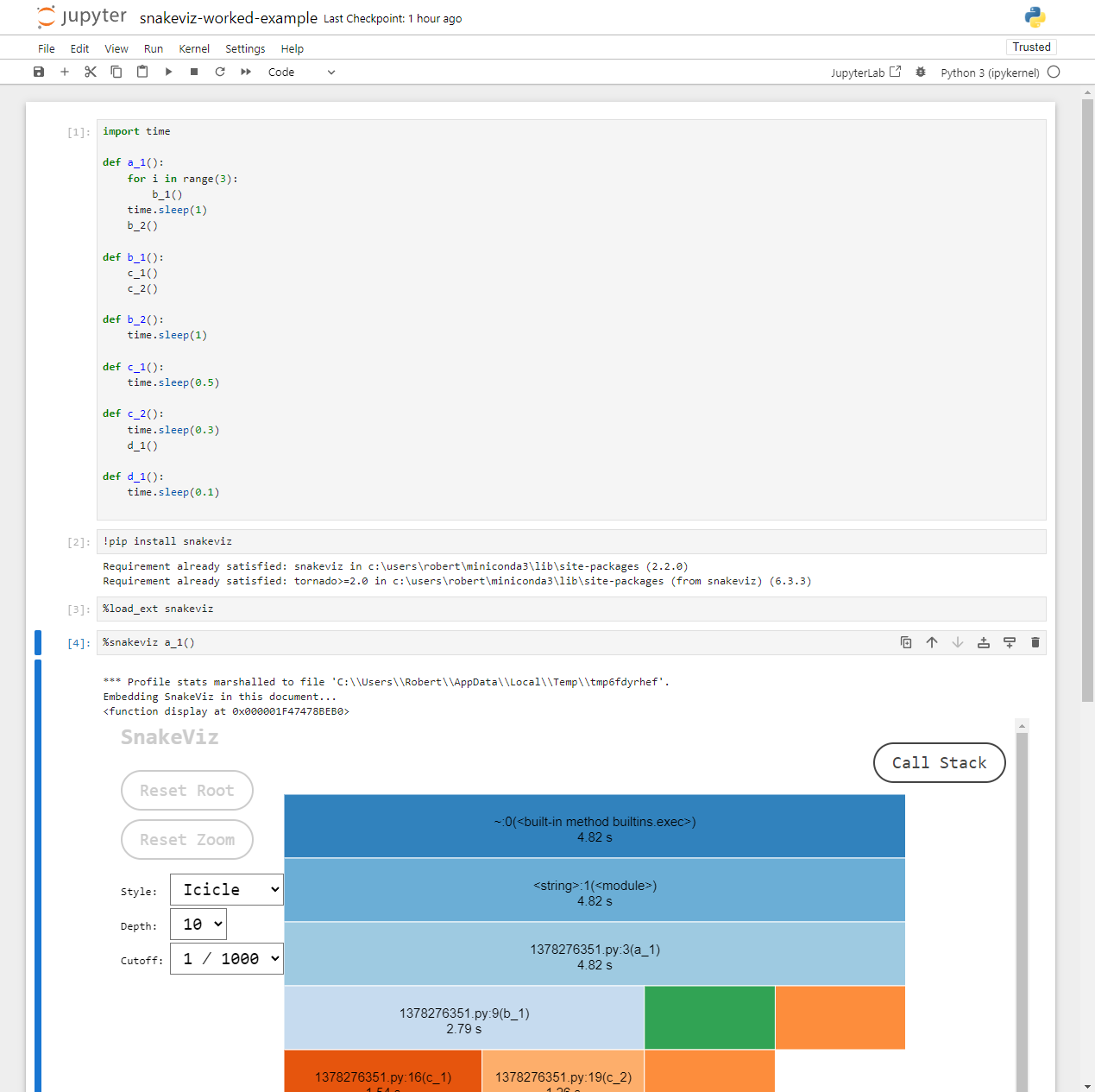
Because notebooks operate by creating temporary Python files, the
filename (shown 1378276351.py above) and line numbers
displayed are not too useful. However, the function names match those
defined in the code and follow the temporary file name in parentheses,
e.g. 1378276351.py:3(a_1),
1378276351.py:9(b_1) refer to the functions
a_1() and b_1() respectively.
Sunburst
snakeviz provides an alternate “Sunburst” visualisation,
accessed via the “Style” drop-down on the left-hand side.
This provides the same information as “Icicle”, however the rows are instead circular with the root method call found at the center.
The sunburst visualisation displays less text on the boxes, so it can be harder to interpret. However, it increases the visibility of boxes further from the root call.

snakeviz for the worked example’s Python code.Exercises
The following exercises allow you to review your understanding of what has been covered in this episode.
Arguments 1-9 passed to travellingsales.py should
execute relatively fast (less than a minute)
This will be slower via the profiler, and is likely to vary on different hardware.
Larger values should be avoided.
Download the set of profiles for arguments 1-10, these can be opened
by passing the directory to snakeviz.
Exercise 1: Travelling Salesperson
Download and profile this Python program, try to locate the function call(s) where the majority of execution time is being spent.
The travelling salesperson problem aims to optimise the route for a scenario where a salesperson is requires to travel between N locations. They wish to travel to each location exactly once, in any order, whilst minimising the total distance travelled.
The provided implementation uses a naive brute-force approach.
The program can be executed via
python travellingsales.py <cities>. The value of
cities should be a positive integer, this algorithm has
poor scaling so larger numbers take significantly longer to run.
- If a hotspot isn’t visible with the argument
1, try increasing the value. - If you think you identified the hotspot with your first profile, try
investigating how the value of
citiesaffects the hotspot within the profile.
The hotspot only becomes visible when an argument of 5
or greater is passed.
You should see that distance() (from
travellingsales.py:11) becomes the largest box (similarly
it’s parent in the call-stack total_distance()) showing
that it scales poorly with the number of cities. With 5 cities,
distance() has a cumulative time of ~35% the
runtime, this increases to ~60% with 9 cities.
Other boxes within the diagram correspond to the initialisation of imports, or initialisation of cities. These have constant or linear scaling, so their cost barely increases with the number of cities.
This highlights the need to profile a realistic test-case expensive enough that initialisation costs are not the most expensive component.
The default configuration of the Predator Prey model takes around 10 seconds to run, it may be slower on other hardware.
Download the pre-generated cProfile output, this can be
opened with snakeviz to save waiting for the profiler.
Exercise 2: Predator Prey
Download and profile the Python predator prey model, try to locate the function call(s) where the majority of execution time is being spent
This exercise uses the packages numpy and
matplotlib, they can be installed via
pip install numpy matplotlib.
The predator prey model is a simple agent-based model of population dynamics. Predators and prey co-exist in a common environment and compete over finite resources.
The three agents; predators, prey and grass exist in a two dimensional grid. Predators eat prey, prey eat grass. The size of each population changes over time. Depending on the parameters of the model, the populations may oscillate, grow or collapse due to the availability of their food source.
The program can be executed via
python predprey.py <steps>. The value of
steps for a full run is 250, however a full run may not be
necessary to find the bottlenecks.
When the model finishes it outputs a graph of the three populations
predprey_out.png.
It should be clear from the profile that the method
Grass::eaten() (from predprey.py:278) occupies
the majority of the runtime.
From the table below the Icicle diagram, we can see that it was called 1,250,000 times.
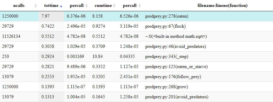
If the table is ordered by ncalls, it can be identified
as the joint 4th most called method and 2nd most called method from
predprey.py.
If you checked predprey_out.png (shown below), you
should notice that there are significantly more Grass
agents than Predators or Prey.
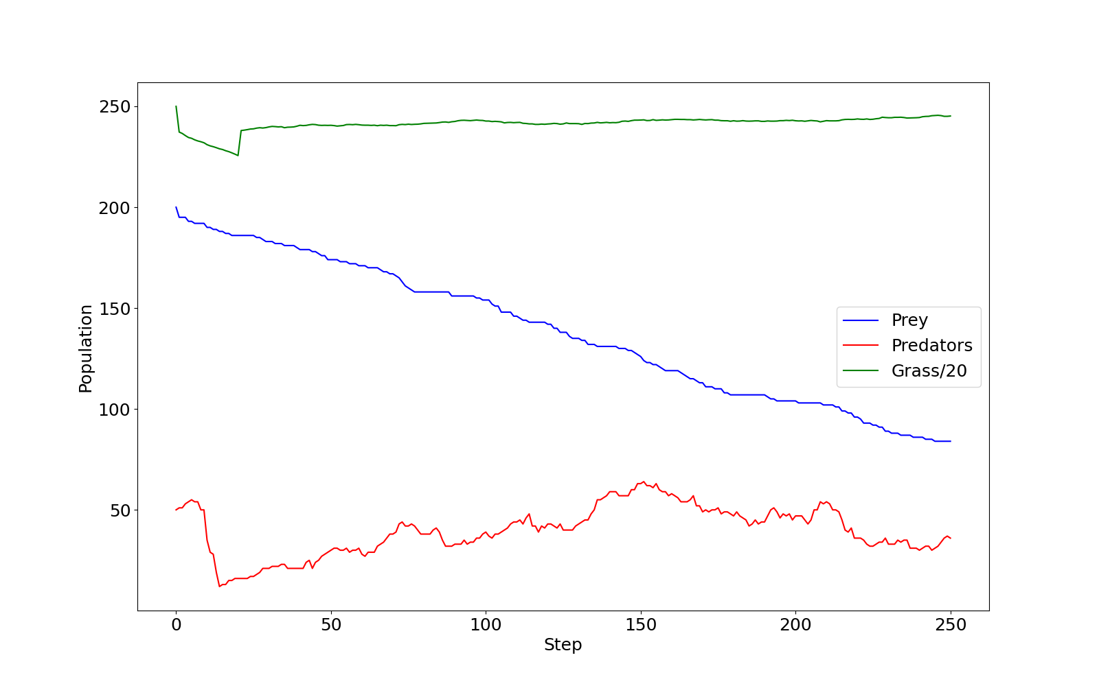
predprey_out.png as produced by the
default configuration of predprey.py.Similarly, the Grass::eaten() has a percall
time is inline with other agent functions such as
Prey::flock() (from predprey.py:67).
Maybe we could investigate this further with line profiling!
You may have noticed many iciles on the right hand of the
diagram, these primarily correspond to the import of
matplotlib which is relatively expensive!
- A python program can be function level profiled with
cProfileviapython -m cProfile -o <output file> <script name> <arguments>. - The output file from
cProfilecan be visualised withsnakevizviapython -m snakeviz <output file>. - Function level profiling output displays the nested call hierarchy, listing both the cumulative and total minus sub functions time.
Content from Break
Last updated on 2024-03-28 | Edit this page
Estimated time: 0 minutes
Take a break. If you can, move around and look at something away from your screen to give your eyes a rest and a chance to absorb the content covered so far.
Content from Line Level Profiling
Last updated on 2025-05-11 | Edit this page
Estimated time: 50 minutes
Overview
Questions
- When is line level profiling appropriate?
- What adjustments are required to Python code to profile with
line_profiler? - How can
kernprofbe used to profile a Python program?
Objectives
- decorate Python code to prepare it for profiling with
line_profiler - execute a Python program via
kernprofto collect profiling information about a Python program’s execution - interpret output from
line_profiler, to identify the lines where time is being spent during a program’s execution
Introduction
Whilst profiling, you may find that function-level profiling highlights expensive methods where you can’t easily determine the cause of the cost due to their complexity.
Line level profiling allows you to target specific methods to collect more granular metrics, which can help narrow the source of expensive computation further. Typically, line-level profiling will calculate the number of times each line is called and the total time spent executing each line. However, with the increased granularity come increased collection costs, which is why it’s targeted to specific methods.
This allows lines that occupy a disproportionate amount of the total runtime to be quickly identified and investigated.
In this episode we will cover the usage of the line-level profiler
line_profiler, how your code should be modified to target
the profiling and how the output can be interpreted.
line_profiler
line_profiler
is a line-level profiler which provides both text output and
visualisation.
It is not part of the Python standard library, and therefore must be installed via pip.
To use line_profiler decorate methods to be profiled
with @profile which is imported from
line_profiler.
For example, the below code:
PYTHON
def is_prime(number):
    if number < 2:
        return False
    for i in range(2, int(number**0.5) + 1):
        if number % i == 0:
            return False
    return True

print(is_prime(1087))
Would be updated to:
PYTHON
from line_profiler import profile

@profile
def is_prime(number):
    if number < 2:
        return False
    for i in range(2, int(number**0.5) + 1):
        if number % i == 0:
            return False
    return True

print(is_prime(1087))
This tells line_profiler to collect metrics for the
lines within the method is_prime(). You can still execute
your code as normal, and these changes will have no effect.
Similar to the earlier tools, line_profiler can then be
triggered via kernprof.
This will output a table per profiled method to console:
OUTPUT
Wrote profile results to my_script.py.lprof
Timer unit: 1e-06 s

Total time: 1.65e-05 s
File: my_script.py
Function: is_prime at line 3

Line #      Hits         Time  Per Hit   % Time  Line Contents
==============================================================
     3                                           @profile
     4                                           def is_prime(number):
     5         1          0.4      0.4      2.4      if number < 2:
     6                                                   return False
     7        32          8.4      0.3     50.9      for i in range(2, int(number**0.5) + 1):
     8        31          7.4      0.2     44.8          if number % i == 0:
     9                                                       return False
    10         1          0.3      0.3      1.8      return True
The columns have the following definitions:
| Column | Definition |
|---|---|
Line # |
The line number of the relevant line within the file (specified above the table). |
Hits |
The total number of times the line was executed. |
Time |
The total time spent executing that line, including child function calls. |
Per Hit |
The average time per call, including child function calls
(Time/Hits). |
% Time |
The time spent executing the line, including child function calls, relative to the other lines of the function. |
Line Contents |
A copy of the line from the file. |
As line_profiler must be attached to specific methods
and cannot attach to a full Python file or project, if your Python file
has significant code in the global scope it will be necessary to move it
into a new method which can then instead be called from global
scope.
The profile is also output to file, in this case
my_script.py.lprof. This file is not human-readable, but
can be printed to console by passing it to line_profiler,
which will then display the same table as above.
Worked Example
Follow Along
Download the Python source for the example and follow along with the worked example on your own machine.
To more clearly demonstrate how to use line_profiler,
the below implementation of “FizzBuzz” will be line profiled.
PYTHON
n = 100
for i in range(1, n + 1):
    if i % 3 == 0 and i % 5 == 0:
        print("FizzBuzz")
    elif i % 3 == 0:
        print("Fizz")
    elif i % 5 == 0:
        print("Buzz")
    else:
        print(i)
As there are no methods, firstly it should be updated to move the code to be profiled into a method:
PYTHON
def fizzbuzz(n):
    for i in range(1, n + 1):
        if i % 3 == 0 and i % 5 == 0:
            print("FizzBuzz")
        elif i % 3 == 0:
            print("Fizz")
        elif i % 5 == 0:
            print("Buzz")
        else:
            print(i)

fizzbuzz(100)
Next the method can be decorated with @profile which
must be imported via line_profiler:
PYTHON
from line_profiler import profile

@profile
def fizzbuzz(n):
    for i in range(1, n + 1):
        if i % 3 == 0 and i % 5 == 0:
            print("FizzBuzz")
        elif i % 3 == 0:
            print("Fizz")
        elif i % 5 == 0:
            print("Buzz")
        else:
            print(i)

fizzbuzz(100)
Now that the code has been decorated, it can be profiled!
This will output a table per profiled method to console:
If you run this locally it should be highlighted due to
-r passed to kernprof.
OUTPUT
Wrote profile results to fizzbuzz.py.lprof
Timer unit: 1e-06 s

Total time: 0.0021535 s
File: fizzbuzz.py
Function: fizzbuzz at line 3

Line #      Hits         Time  Per Hit   % Time  Line Contents
==============================================================
     3                                           @profile
     4                                           def fizzbuzz(n):
     5       101         32.5      0.3      1.5      for i in range(1, n + 1):
     6       100         26.9      0.3      1.2          if i % 3 == 0 and i % 5 == 0:
     7         6        125.8     21.0      5.8              print("FizzBuzz")
     8        94         16.7      0.2      0.8          elif i % 3 == 0:
     9        27        541.3     20.0     25.1              print("Fizz")
    10        67         12.4      0.2      0.6          elif i % 5 == 0:
    11        14        285.1     20.4     13.2              print("Buzz")
    12                                                   else:
    13        53       1112.8     21.0     51.7              print(i)
For this basic example, we can calculate that “FizzBuzz” would be
printed 6 times out of 100, and the profile shows that line 7
(print("FizzBuzz")) occupied 5.8% of the runtime. This is
slightly lower than 6% due to the control flow code (printing to console
is expensive relative to the control flow and conditional statements).
Similarly, “Fizz” is printed 27 times and occupies 25.1%, likewise
“Buzz” is printed 14 times and occupies 13.2%. Each print statement has
a similar “Per Hit” time of 20-21 micro seconds.
Therefore it can be seen in this example, how the time spent executing each line matches expectations.
Rich Output
The -r argument passed to kernprof (or
line_profiler) enables rich output, if you run the profile
locally it should look similar to this. This requires the optional
package rich, it will have been installed if
[all] was specified when installing
line_profiler with pip.
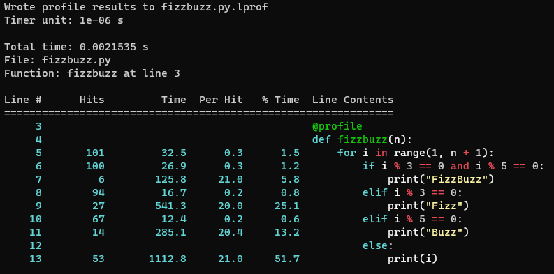
line_profiler for the above FizzBuzz profile code.line_profiler Inside Notebooks
If you’re more familiar with writing Python inside Jupyter notebooks
you can, as with snakeviz, use line_profiler
directly from inside notebooks. However, it is still necessary for the
code you wish to profile to be placed within a function.
First line_profiler must be installed and it’s extension
loaded.
Following this, you call line_profiler with
%lprun.
The functions to be line profiled are specified with
-f <function name>, this is repeated for each
individual function that you would otherwise apply the
@profile decorator to.
This is followed by calling the function which runs the full code to be profiled.
For the above FizzBuzz example it would be:
This will then create an output cell with any output from the
profiled code, followed by the standard output from
line_profiler. It is not currently possible to get the
rich/coloured output from line_profiler within
notebooks.
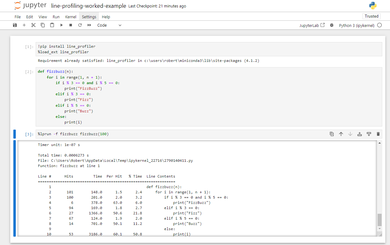
line_profiler
inside a Juypter notebook for the above FizzBuzz profile code.Exercises
The following exercises allow you to review your understanding of what has been covered in this episode.
Exercise 1: BubbleSort
Download and profile the Python bubblesort implementation, line-level profile the code to investigate where time is being spent.
Bubblesort is a basic sorting algorithm, it is not considered to be efficient so in practice other sorting algorithms are typically used.
The array to be sorted is iterated, with a pair-wise sort being applied to each element and it’s neighbour. This can cause elements to rise (or sink) multiple positions in a single pass, hence the name bubblesort. This iteration continues until the array is fully iterated with no elements being swapped.
The program can be executed via
python bubblesort.py <elements>. The value of
elements should be a positive integer as it represents the
number of elements to be sorted.
- Remember that the code needs to be moved into a method decorated
with
@profile - This must be imported via
from line_profiler import profile - 100 elements should be suitable for a quick profile
If you chose to profile the whole code, it may look like this:
PYTHON
import sys
import random
from line_profiler import profile        # Import profile decorator

@profile                                 # Decorate the function to be profiled
def main():                              # Create a simple function with the code to be profiled
    # Argument parsing
    if len(sys.argv) != 2:
        print("Script expects 1 positive integer argument, %u found."%(len(sys.argv) - 1))
        sys.exit()
    n = int(sys.argv[1])
    # Init
    random.seed(12)
    arr = [random.random() for i in range(n)]
    print("Sorting %d elements"%(n))
    # Sort
    for i in range(n - 1):
        swapped = False
        for j in range(0, n - i - 1):
            if arr[j] > arr[j + 1]:
                arr[j], arr[j + 1] = arr[j + 1], arr[j]
                swapped = True
        # If no two elements were swapped in the inner loop, the array is sorted
        if not swapped:
            break
    # Validate
    is_sorted = True
    for i in range(n - 1):
        if arr[i] > arr[i+1]:
            is_sorted = False
    print("Sorting: %s"%("Passed" if is_sorted else "Failed"))

main()                                  # Call the created function
The sort can be profiled with 100 elements, this is quick and should be representative.
This produces output:
OUTPUT
Wrote profile results to bubblesort.py.lprof
Timer unit: 1e-06 s

Total time: 0.002973 s
File: bubblesort.py
Function: main at line 5

Line #      Hits         Time  Per Hit   % Time  Line Contents
==============================================================
     5                                           @profile
     6                                           def main():
     7                                               # Argument parsing
     8         1          0.7      0.7      0.0      if len(sys.argv) != 2:
     9                                                   print("Script expects 1 positive integer argument, %u found."%…
    10                                                   sys.exit()
    11         1          1.6      1.6      0.1      n = int(sys.argv[1])
    12                                               # Init
    13         1          8.8      8.8      0.3      random.seed(12)
    14         1         16.6     16.6      0.6      arr = [random.random() for i in range(n)]
    15         1         38.2     38.2      1.3      print("Sorting %d elements"%(n))
    16                                               # Sort
    17        95         14.5      0.2      0.5      for i in range(n - 1):
    18        95         13.1      0.1      0.4          swapped = False
    19      5035        723.1      0.1     24.3          for j in range(0, n - i - 1):
    20      4940       1045.9      0.2     35.2              if arr[j] > arr[j + 1]:
    21      2452        686.9      0.3     23.1                  arr[j], arr[j + 1] = arr[j + 1], arr[j]
    22      2452        353.0      0.1     11.9                  swapped = True
    23                                                   # If no two elements were swapped in the inner loop, the array…
    24        95         15.2      0.2      0.5          if not swapped:
    25         1          0.2      0.2      0.0              break
    26                                               # Validate
    27         1          0.5      0.5      0.0      is_sorted = True
    28       100         12.9      0.1      0.4      for i in range(n - 1):
    29        99         20.3      0.2      0.7          if arr[i] > arr[i+1]:
    30                                                       is_sorted = False
    31         1         21.5     21.5      0.7      print("Sorting: %s"%("Passed" if is_sorted else "Failed"))
From this we can identify that the print statements were the most expensive individual calls (“Per Hit”), however both were only called once. Most execution time was spent at the inner loop (lines 19-22).
As this is a reference implementation of a classic sorting algorithm we are unlikely to be able to improve it further.
Download the pre-generated line_profiler output, this
can be opened be to save waiting for the profiler.
Exercise 2: Predator Prey
During the function-level profiling episode,
the Python predator prey
model was function-level profiled. This highlighted that
Grass::eaten() (from predprey.py:278) occupies
the majority of the runtime.
Line-profile this method, using the output from the profile consider how it might be optimised.
- Remember that the function needs to be decorated with
@profile - This must be imported via
from line_profiler import profile - Line-level profiling
Grass::eaten(), the most called function will slow it down significantly. You may wish to reduce the number of stepspredprey.py:305.
First the function must be decorated
line_profiler can then be executed via
python -m kernprof -lvr predprey.py <steps>.
Since this will take much longer to run due to
line_profiler, you may wish to profile fewer
steps than you did in the function-level profiling exercise
(250 was suggested for a full run). In this instance it may change the
profiling output slightly, as the number of Prey and their
member variables evaluated by this method both change as the model
progresses, but the overall pattern is likely to remain similar.
Alternatively, you can kill the profiling process
(e.g. ctrl + c) after a minute and the currently collected
partial profiling information will be output.
This will produce output similar to that below.
OUTPUT
Wrote profile results to predprey.py.lprof
Timer unit: 1e-06 s

Total time: 101.573 s
File: predprey.py
Function: eaten at line 278

Line #      Hits         Time  Per Hit   % Time  Line Contents
==============================================================
   278                                               @profile
   279                                               def eaten(self, prey_list):
   280   1250000     227663.1      0.2      0.2          if self.available:
   281   1201630     165896.4      0.1      0.2              prey_index = -1
   282   1201630     166219.0      0.1      0.2              closest_prey = GRASS_EAT_DISTANCE
   283
   284                                                       # Iterate prey_location messages to find the closest prey
   285 198235791   29227902.1      0.1     28.8              for i in range(len(prey_list)):
   286 197034161   30158318.8      0.2     29.7                  prey = prey_list[i]
   287 197034161   38781451.1      0.2     38.2                  if prey.life < PREY_HUNGER_THRESH:
   288                                                               # Check if they are within interaction radius
   289   2969470     579923.4      0.2      0.6                      dx = self.x - prey.x
   290   2969470     552092.2      0.2      0.5                      dy = self.y - prey.y
   291   2969470     938669.8      0.3      0.9                      distance = math.sqrt(dx*dx + dy*dy)
   292
   293   2969470     552853.8      0.2      0.5                      if distance < closest_prey:
   294      2532        469.3      0.2      0.0                          prey_index = i
   295      2532        430.1      0.2      0.0                          closest_prey = distance
   296
   297   1201630     217534.5      0.2      0.2              if prey_index >= 0:
   298                                                           # Add grass eaten message
   299      2497       2181.8      0.9      0.0                  prey_list[prey_index].life += GAIN_FROM_FOOD_PREY
   300
   301                                                           # Update grass agent variables
   302      2497        793.9      0.3      0.0                  self.dead_cycles = 0
   303      2497        631.0      0.3      0.0                  self.available = 0
From the profiling output it can be seen that lines 285-287 occupy over 90% of the method’s runtime!
Given that the following line 289 only has a relative 0.6% time, it
can be understood that the vast majority of times the condition
prey.life < PREY_HUNGER_THRESH is evaluated it does not
proceed.
Remembering that this method is executed once per each of the 5000
Grass agents each step of the model, it could make sense to
pre-filter prey_list once each time-step before it is
passed to Grass::eaten(). This would greatly reduce the
number of Prey iterated, reducing the cost of the
method.
- Specific methods can be line-level profiled if decorated with
@profilethat is imported fromline_profiler. -
kernprofexecutesline_profilerviapython -m kernprof -lvr <script name> <arguments>. - Code in global scope must be wrapped in a method if it is to be
profiled with
line_profiler. - The output from
line_profilerlists the absolute and relative time spent per line for each targeted function.
Content from Profiling Conclusion
Last updated on 2024-03-28 | Edit this page
Estimated time: 5 minutes
Overview
Questions
- What has been learnt about profiling?
Objectives
- Review what has been learnt about profiling
This concludes the profiling portion of the course.
cProfile, snakeviz and
line_profiler have been introduced, these are some of the
most accessible Python profiling tools.
With these transferable skills, if necessary, you should be able to
follow documentation to use more advanced Python profiling tools such as
scalene.
What profiling is:
- The collection and analysis of metrics relating to the performance of a program during execution .
Why programmers can benefit from profiling:
- Narrows down the costly areas of code, allowing optimisation to be prioritised or decided to be unnecessary.
When to Profile:
- Profiling should be performed on functional code, either when concerned about performance or prior to release/deployment.
What to Profile:
- The collection of profiling metrics will often slow the execution of code, therefore the test-case should be narrow whilst remaining representative of a realistic run.
How to function-level profile:
- Execute
cProfileviapython -m cProfile -o <output file> <script name> <arguments> - Execute
snakevizviapython -m snakeviz <output file>
How to line-level profile:
- Import
profilefromline_profiling - Decorate targeted methods with
@profile - Execute
line_profilerviapython -m kernprof -lvr <script name> <arguments>
Content from Introduction to Optimisation
Last updated on 2025-03-26 | Edit this page
Estimated time: 10 minutes
Overview
Questions
- Why could optimisation of code be harmful?
Objectives
- Able to explain the cost benefit analysis of performing code optimisation
Introduction
Now that you’re able to find the most expensive components of your code with profiling, we can think about ways to improve it. However, the best way to do this will depend a lot on your specific code! For example, if your code is spending 60 seconds waiting to download data files and then 1 second to analyse that data, then optimizing your data analysis code won’t make much of a difference. We’ll talk briefly about some of these external bottlenecks at the end. For now, we’ll assume that you’re not waiting for anything else and we’ll look at the performance of your code.
In order to optimise code for performance, it is necessary to have an understanding of what a computer is doing to execute it.
A high-level understanding of how your code executes, such as how Python and the most common data-structures and algorithms are implemented, can help you identify suboptimal approaches when programming. If you have learned to write code informally out of necessity, to get something to work, it’s not uncommon to have collected some “unpythonic” habits along the way that may harm your code’s performance.
These are the first steps in code optimisation, and knowledge you can put into practice by making more informed choices as you write your code and after profiling it.
The remaining content is often abstract knowledge, that is transferable to the vast majority of programming languages. This is because the hardware architecture, data-structures and algorithms used are common to many languages and they hold some of the greatest influence over performance bottlenecks.
Performance vs Maintainability
Programmers waste enormous amounts of time thinking about, or worrying about, the speed of noncritical parts of their programs, and these attempts at efficiency actually have a strong negative impact when debugging and maintenance are considered. We should forget about small efficiencies, say about 97% of the time: premature optimization is the root of all evil. Yet we should not pass up our opportunities in that critical 3%. - Donald Knuth
This classic quote among computer scientists emphasises the importance of considering both performance and maintainability when optimising code and prioritising your optimisations.
While advanced optimisations may boost performance, they often come at the cost of making the code harder to understand and maintain. Even if you’re working alone on private code, your future self should be able to easily understand the implementation. Hence, when optimising, always weigh the potential impact on both performance and maintainability. While this course does not cover most advanced optimisations, you may already be familiar with and using some.
Profiling is a valuable tool for prioritising optimisations. Should effort be expended to optimise a component which occupies 1% of the runtime? Or would that time be better spent optimising the most expensive components?
This doesn’t mean you should ignore performance when initially writing code. Choosing the right algorithms and data structures, as we will discuss in this course, is good practice. However, there’s no need to obsess over micro-optimising every tiny component of your code—focus on the bigger picture.
Performance of Python
If you’ve read about different programming languages, you may have heard that there’s a difference between “interpreted” languages (like Python) and “compiled” languages (like C). You may have heard that Python is slow because it is an interpreted language. To understand where this comes from (and how to get around it), let’s talk a little bit about how Python works.
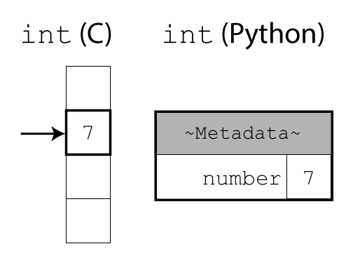
In C, integers (or other basic types) are raw data in memory. It is up to the programmer to keep track of the data type. The compiler can then turn the source code directly into machine code. This allows the compiler to perform low-level optimisations that better exploit hardware nuance to achieve fast performance. This however comes at the cost of compiled software not being cross-platform.
In Python, everything is a complex object. The interpreter uses extra fields in the header to keep track of data types at runtime or take care of memory management. This adds a lot more flexibility and makes life easier for programmers. However, it comes at the cost of some overhead in both time and memory usage.
Objects store both their raw data (like an integer or string) and
some internal information used by the interpreter. We can see that
additional storage space with sys.getsizeof(), which shows
how many bytes an object takes up:
PYTHON
import sys

sys.getsizeof("")  # 41
sys.getsizeof("a")  # 42
sys.getsizeof("ab")  # 43

sys.getsizeof([])  # 56
sys.getsizeof(["a"])  # 64

sys.getsizeof(1)  # 28
(Note: For container objects (like lists and dictionaries) or custom
classes, values returned by getsizeof() are
implementation-dependent and may not reflect the actual memory
usage.)
We effectively gain programmer performance by sacrificing some code performance. Most of the time, computers are “fast enough” so this is the right trade-off, as Donald Knuth said.
However, there are the few other cases where code performance really matters. To handle these cases, Python has the capability to integrate with code written in lower-level programming language (like C, Fortran or Rust) under the hood. Some performance-sensitive libraries therefore perform a lot of the work in such low-level code, before returning a nice Python object back to you. (We’ll discuss NumPy in a later section; but many parts of the Python standard library also use this pattern.)
Therefore, it is often best to tell the interpreter/library at a high level what you want, and let it figure out how to do it.
That way, the interpreter/library is free to do all its work in the low-level code, and adds overhead only once, when it creates and returns a Python object in the end. This usually makes your code more readable, too: When someone else reads your code, they can see exactly what you want to do, without getting overwhelmed by overly detailed step-by-step instructions.
Ensuring Reproducible Results
When optimising existing code, you’re often making speculative changes, which can lead to subtle mistakes. To ensure that your optimisations aren’t also introducing errors, it’s crucial to have a strategy for checking that the results remain correct.
Testing should already be an integral part of your development process. It helps clarify expected behaviour, ensures new features are working as intended, and protects against unintended regressions in previously working functionality. Always verify your changes through testing to ensure that the optimisations don’t compromise the correctness of your code.
pytest Overview
There are a plethora of methods for testing code. Most Python developers use the testing package pytest, it’s a great place to get started if you’re new to testing code.
Here’s a quick example of how a test can be used to check your function’s output against an expected value.
Tests should be created within a project’s testing directory, by
creating files named with the form test_*.py or
*_test.py. pytest looks for file names with these patterns
when running the test suite.
Within the created test file, any functions named in the form
test* are considered tests that will be executed by
pytest.
The assert keyword is used, to test whether a condition
evaluates to True.
PYTHON
# file: test_demonstration.py

# A simple function to be tested, this could instead be an imported package
def squared(x):
    return x**2

# A simple test case
def test_example():
    assert squared(5) == 24
When py.test is called inside a working directory, it
will then recursively find and execute all the available tests.
SH
>py.test
================================================= test session starts =================================================
platform win32 -- Python 3.10.12, pytest-7.3.1, pluggy-1.3.0
rootdir: C:\demo
plugins: anyio-4.0.0, cov-4.1.0, xdoctest-1.1.2
collected 1 item

test_demonstration.py F                                                                                          [100%]

====================================================== FAILURES =======================================================
____________________________________________________ test_example _____________________________________________________

    def test_example():
>       assert squared(5) == 24
E       assert 25 == 24
E        +  where 25 = squared(5)

test_demonstration.py:9: AssertionError
=============================================== short test summary info ===============================================
FAILED test_demonstration.py::test_example - assert 25 == 24
================================================== 1 failed in 0.07s ==================================================
Whilst not designed for benchmarking, it does provide the total time the test suite took to execute. In some cases this may help identify whether the optimisations have had a significant impact on performance.
This is only the simplest introduction to using pytest, it has advanced features common to other testing frameworks such as fixtures, mocking and test skipping. pytest’s documentation covers all this and more. You may already have a different testing workflow in-place for validating the correctness of the outputs from your code.
- Fixtures: A test fixture is a common class which multiple tests can inherit from. This class will typically include methods that perform common initialisation and teardown actions around the behaviour to be tested. This reduces repeated code.
- Mocking: If you wish to test a feature which would relies on a live or temperamental service, such as making API calls to a website. You can mock that API, so that when the test runs synthetic responses are produced rather than the real API being used.
- Test skipping: You may have configurations of your software that cause certain tests to be unsupported. Skipping allows conditions to be added to tests, to decide whether they should be executed or skipped.
- The knowledge necessary to perform high-level optimisations of code is largely transferable between programming languages.
- When considering optimisation it is important to focus on the potential impact, both to the performance and maintainability of the code.
- Many high-level optimisations should be considered good-practice.
Content from Using Python Language Features and the Standard Library
Last updated on 2025-11-26 | Edit this page
Estimated time: 15 minutes
Overview
Questions
- Why are Python loops slower than specialised functions?
- How can I make my code more readable and faster?
Objectives
- Able to utilise Python language features effectively
- Able to search Python documentation for functionality available in built-in types and in the standard library
- Able to identify when Python code can be rewritten to perform execution in the back-end.
This episode discusses relatively fundamental features of Python.
For students experienced with writing Python, many of these points may be unnecessary. However, self-taught students—especially if they have previously studied lower-level languages with a less powerful standard library—may have adopted “unpythonic” habits and will particularly benefit from this section.
Before we look at data structures, algorithms and third-party libraries, it’s worth reviewing the fundamentals of Python. If you’re familiar with other programming languages, like C or Delphi, you might not know the Pythonic approaches. Whilst you can write Python in a way similar to other languages, it is often more effective to take advantage of Python’s principles and idioms.
Built-in Functions
For example, you might think to sum a list of numbers by using a for
loop, as would be typical in C, as shown in the function
manualSumC() and manualSumPy() below.
PYTHON
import random
from timeit import timeit

N = 100000  # Number of elements in the list

# Ensure every list is the same
random.seed(12)
my_data = [random.random() for i in range(N)]


def manualSumC():
    n = 0
    for i in range(len(my_data)):
        n += my_data[i]
    return n

def manualSumPy():
    n = 0
    for evt_count in my_data:
        n += evt_count
    return n

def builtinSum():
    return sum(my_data)


repeats = 1000
print(f"manualSumC: {timeit(manualSumC, globals=globals(), number=repeats):.3f}ms")
print(f"manualSumPy: {timeit(manualSumPy, globals=globals(), number=repeats):.3f}ms")
print(f"builtinSum: {timeit(builtinSum, globals=globals(), number=repeats):.3f}ms")
Even just replacing the iteration over indices (which may be a habit
you’ve picked up if you first learned to program in C) with a more
pythonic iteration over the elements themselves speeds up the code by
about 2x. But even better, by switching to the built-in
sum() function our code becomes about 8x faster and much
easier to read while doing the exact same operation!
OUTPUT
manualSumC: 1.624ms
manualSumPy: 0.740ms
builtinSum: 0.218ms
This is because built-in functions (i.e. those that are available without importing packages) are typically implemented in the CPython back-end, so their performance benefits from bypassing the Python interpreter.
In particular, those which are passed an iterable
(e.g. lists) are likely to provide the greatest benefits to performance.
The Python documentation provides equivalent Python code for many of
these cases.
-
all(): boolean and of all items -
any(): boolean or of all items -
max(): Return the maximum item -
min(): Return the minimum item -
sum(): Return the sum of all items
This is a nice illustration of the principle we discussed earlier: It is often best to tell the interpreter/library at a high level what you want, and let it figure out how to do it.
Example: Searching an element in a list
A simple example of this is performing a linear search on a list.
(Though as we’ll see in the next section, this isn’t the most efficient
approach!) In the following example, we create a list of 2500 random
integers in the (inclusive-exclusive) range [0, 5000). The
goal is to count how many unique even numbers are in the list.
The function manualSearch() manually iterates through
the list (ls) and checks each individual item using Python
code. On the other hand, operatorSearch() uses the
in operator to perform each search, which allows CPython to
implement the inner loop in its C back-end.
PYTHON
import random
from timeit import timeit

N = 2500  # Number of elements in list
M = 2  # N*M == Range over which the elements span
ls = [random.randint(0, int(N*M)) for i in range(N)]

def manualSearch():
    count = 0
    for even_number in range(0, int(N*M), M):
        for i in range(0, len(ls)):
            if ls[i] == even_number:
                count += 1
                break

def operatorSearch():
    count = 0
    for even_number in range(0, int(N*M), M):
        if even_number in ls:
            count += 1

repeats = 1000
print(f"manualSearch: {timeit(manualSearch, number=repeats):.2f}ms")
print(f"operatorSearch: {timeit(operatorSearch, number=repeats):.2f}ms")
This results in the manual Python implementation being 5x slower, doing the exact same operation!
OUTPUT
manualSearch: 152.15ms
operatorSearch: 28.43ms
An easy approach to follow is that if two blocks of code do the same operation, the one that contains less Python is probably faster. This won’t apply if you’re using 3rd party packages written purely in Python though.
Example: Parsing data from a text file
In C, since there is no high-level string datatype,
parsing strings can be fairly arduous work where you repeatedly look for
the index of a separator character in the string and use that index to
split the string up.
Challenge
Let’s say we have read in some data from a text file, each line containing a time bin and a mean energy:
If you’ve a C programming background, you may write the following code to parse the data into a dictionary:
PYTHON
def manualSplit():
    data = {}
    for line in f:
        first_char = line.find("0")
        end_time = line.find(" ", first_char, -1)

        energy_found = line.find(".", end_time, -1)
        begin_energy = line.rfind(" ", end_time, energy_found)
        end_energy = line.find(" ", energy_found)
        if end_energy == -1:
            end_energy = len(line)

        time = line[first_char:end_time]
        energy = line[begin_energy + 1:end_energy]

        data[time] = energy
    return data
Can you find a shorter, more easily understandable way to write this in Python?
Python strings have a lot of methods to perform common operations, like removing suffixes, replacing substrings, joining or splitting, stripping whitespaces, and much more. See Python’s string methods documentation for a full list.
PYTHON
def builtinSplit():
    data = {}
    for line in f:
        time, energy = line.split()
        data[time] = energy
    return data
This code is not just much more readable; it is also more flexible,
since it does not rely on the precise formatting of the input strings.
(For example, the line first_char = line.find("0") in the
original code assumes that the time bin starts with the digit 0. That
code would likely malfunction if the input file had more than 1000 time
bins.)
The code that’s executed by CPython may use a similar approach as in
manualSplit(); however, since this is all happening “under
the hood” in C code, it is once again faster.
PYTHON
N = 10_000  # Number of elements in the list

# Ensure every list is the same
random.seed(12)
f = [f" {i:0>6d} {random.random():8.4f} " for i in range(N)]

repeats = 1000
print(f"manualSplit: {timeit(manualSplit, globals=globals(), number=repeats):.3f}ms")
print(f"builtinSplit: {timeit(builtinSplit, globals=globals(), number=repeats):.3f}ms")
OUTPUT
manualSplit: 1.797ms
builtinSplit: 0.796ms
Challenge
If you’ve brought a project you want to work on: Do you have any similar code in there, which is hard to understand because it contains a lot of low-level step-by-step instructions?
(Before you try to rewrite those parts of your code, use a profiler to see whether those parts have a noticeable impact on the overall performance of your project. Remember the Donald Knuth quote!)
Content from Data Structures & Algorithms
Last updated on 2025-11-26 | Edit this page
Estimated time: 35 minutes
Overview
Questions
- What’s the most efficient way to construct a list?
- When should tuples be used?
- When are sets appropriate?
- What is the best way to search a list?
Objectives
- Able to summarise how lists and tuples work behind the scenes.
- Able to identify appropriate use-cases for tuples.
- Able to utilise dictionaries and sets effectively
- Able to use
bisect_left()to perform a binary search of a list or array
The important information for students to learn within this episode are the patterns demonstrated via the benchmarks.
This episode introduces many complex topics, these are used to ground the performant patterns in understanding to aid memorisation.
It should not be a concern to students if they find the data-structure/algorithm internals challenging, if they are still able to recognise the demonstrated patterns.
This episode is challenging!
Within this episode you will be introduced to how certain data-structures and algorithms work.
This is used to explain why one approach is likely to execute faster than another.
It matters that you are able to recognise the faster/slower approaches, not that you can describe or reimplement these data-structures and algorithms yourself.
Lists
Lists are a fundamental data structure within Python.
It is implemented as a form of dynamic array found within many
programming languages by different names (C++: std::vector,
Java: ArrayList, R: vector, Julia:
Vector).
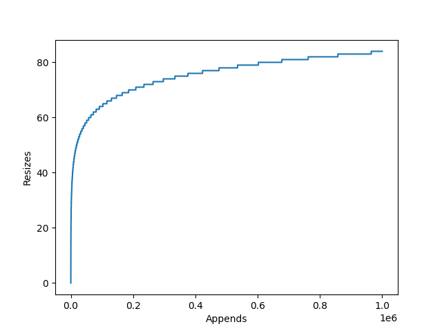
They allow direct and sequential element access, with the convenience to append items.
This is achieved by internally storing items in a static array. This array however can be longer than the list, so the current length of the list is stored alongside the array. When an item is appended, the list checks whether it has enough spare space to add the item to the end. If it doesn’t, it will re-allocate a larger array, copy across the elements, and deallocate the old array. The item to be appended is then copied to the end and the counter which tracks the list’s length is incremented.
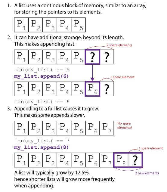
The amount the internal array grows by is dependent on the particular
list implementation’s growth factor. CPython for example uses newsize + (newsize >> 3) + 6,
which works out to an over allocation of roughly ~12.5%.
This has two implications:
- If you are growing a list with
append(), there will be large amounts of redundant allocations and copies as the list grows. - The resized list may use up to 12.5% excess memory.
List Comprehension
If creating a list via append() is undesirable, the
natural alternative is to use list-comprehension.
List comprehension can be twice as fast at building lists than using
append(). This is primarily because list-comprehension
allows Python to offload much of the computation into faster C code.
General Python loops in contrast can be used for much more, so they
remain in Python bytecode during computation which has additional
overheads.
This can be demonstrated with the below benchmark:
PYTHON
from timeit import timeit

def list_append():
    li = []
    for i in range(100000):
        li.append(i)

def list_preallocate():
    li = [0]*100000
    for i in range(100000):
        li[i] = i

def list_comprehension():
    li = [i for i in range(100000)]

repeats = 1000
print(f"Append: {timeit(list_append, number=repeats):.2f}ms")
print(f"Preallocate: {timeit(list_preallocate, number=repeats):.2f}ms")
print(f"Comprehension: {timeit(list_comprehension, number=repeats):.2f}ms")
timeit is used to run each function 1000 times,
providing the below averages:
OUTPUT
Append: 3.50ms
Preallocate: 2.48ms
Comprehension: 1.69ms
Results will vary between Python versions, hardware and list lengths. But in this example list comprehension was 2x faster, with pre-allocate fairing in the middle. Although this is milliseconds, this can soon add up if you are regularly creating lists.
Tuples
In contrast to lists, Python’s tuples are immutable static arrays (similar to strings): Their elements cannot be modified and they cannot be resized.
Their potential use-cases are greatly reduced due to these two limitations, they are only suitable for groups of immutable properties.
Tuples can still be joined with the + operator, similar
to appending lists, however the result is always a newly allocated tuple
(without a list’s over-allocation).
Python caches a large number of short (1-20 element) tuples. This greatly reduces the cost of creating and destroying them during execution at the cost of a slight memory overhead.
This can be easily demonstrated with Python’s timeit
module in your console.
SH
>python -m timeit "li = [0,1,2,3,4,5]"
10000000 loops, best of 5: 26.4 nsec per loop

>python -m timeit "tu = (0,1,2,3,4,5)"
50000000 loops, best of 5: 7.99 nsec per loop
It takes 3x as long to allocate a short list than a tuple of equal length. This gap only grows with the length, as the tuple cost remains roughly static whereas the cost of allocating the list grows slightly.
Dictionaries
Dictionaries are another fundamental Python data-structure. They provide a key-value store, whereby unique keys with no intrinsic order map to attached values.
“no intrinsic order”
Since Python 3.6, the items within a dictionary will iterate in the order that they were inserted. This does not apply to sets.
OrderedDict still exists, and may be preferable if the
order of items is important when performing whole-dictionary
equality.
Hashing Data Structures
Python’s dictionaries are implemented as hashing data structures, we can understand these at a high-level with an analogy:
A Python list is like having a single long bookshelf. When you buy a new book (append a new element to the list), you place it at the far end of the shelf, right after all the previous books.

A Python dictionary is more like a bookcase with several shelves, labelled by genre (sci-fi, romance, children’s books, non-fiction, …) and author surname. When you buy a new book by Jules Verne, you might place it on the shelf labelled "Sci-Fi, V–Z". And if you keep adding more books, at some point you’ll move to a larger bookcase with more shelves (and thus more fine-grained sorting), to make sure you don’t have too many books on a single shelf.
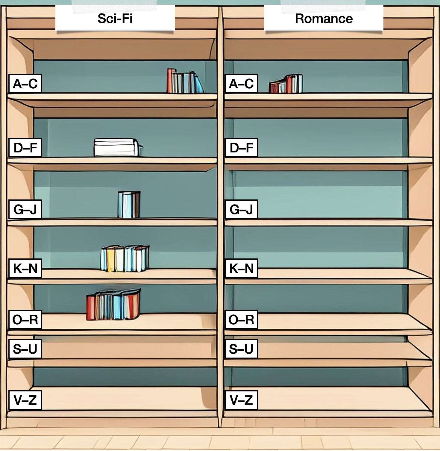
Now, let’s say a friend wanted to borrow the book "‘—All You Zombies—’" by Robert Heinlein. If I had my books arranged on a single bookshelf (in a list), I would have to look through every book I own in order to find it. However, if I had a bookcase with several shelves (a hashing data structure), I know immediately that I need to check the shelf "Sci-Fi, G—J", so I’d be able to find it much more quickly!
The large bookcases in the second illustration, with many shelves almost empty, take up a lot more space than the single shelf in the first illustration. This may also be interpreted as the dictionary using more memory than a list.
In principle, this is correct. However:
- The actual difference is much less pronounced than in the illustration. (A list requires about 8 bytes to keep track of each item, while a dictionary requires about 30 bytes.)
- In most cases this net size of the list/dictionary itself is negligibly small compared to the size of the objects stored in the list or dictionary (e.g. 41 bytes for an empty string or 112 bytes for an empty NumPy array).
In practice, therefore, this trade-off between memory usage and speed is usually worth it.
When a value is inserted into a dictionary, its key is hashed to decide on which “shelf” it should be stored. Most items will have a unique shelf, allowing them to be accessed directly. This is typically much faster for locating a specific item than searching a list.
Keys
A dictionary’s keys will typically be a core Python type such as a
number or string. However, multiple of these can be combined as a tuple
to form a compound key, or a custom class can be used if the methods
__hash__() and __eq__() have been
implemented.
You can implement __hash__() by utilising the ability
for Python to hash tuples, avoiding the need to implement a bespoke hash
function.
PYTHON
class MyKey:

    def __init__(self, _a, _b, _c):
        self.a = _a
        self.b = _b
        self.c = _c

    def __eq__(self, other):
        return (isinstance(other, type(self))
                and (self.a, self.b, self.c) == (other.a, other.b, other.c))

    def __hash__(self):
        return hash((self.a, self.b, self.c))

dict = {}
dict[MyKey("one", 2, 3.0)] = 12
The only limitation is that where two objects are equal they must
have the same hash, hence all member variables which contribute to
__eq__() should also contribute to __hash__()
and vice versa (it’s fine to have irrelevant or redundant internal
members contribute to neither).
Sets
Sets are dictionaries without the values (both are declared using
{}), a collection of unique keys equivalent to the
mathematical set. Modern CPython now uses a set implementation
distinct from that of it’s dictionary, however they still behave much
the same in terms of performance characteristics.
Sets are used for eliminating duplicates and checking for membership, and will normally outperform lists especially when the list cannot be maintained sorted.
Exercise: Unique Collection
There are four implementations in the below example code, each builds a collection of unique elements from 25,000 where 50% can be expected to be duplicates.
Estimate how the performance of each approach is likely to stack up.
If you reduce the value of repeats it will run faster,
how does changing the number of items (N) or the ratio of
duplicates int(N/2) affect performance?
PYTHON
import random
from timeit import timeit

N = 25000  # Number of elements in the list
data = [random.randint(0, int(N/2)) for i in range(N)]

def uniqueSet():
    set_out = set(data)

def uniqueSetAdd():
    set_out = set()
    for i in data:
        set_out.add(i)

def uniqueList():
    ls_out = []
    for i in data:
        if not i in ls_out:
            ls_out.append(i)

def uniqueListSort():
    ls_in = sorted(data)
    ls_out = [ls_in[0]]
    for i in ls_in:
        if ls_out[-1] != i:
            ls_out.append(i)

repeats = 1000
print(f"uniqueSet: {timeit(uniqueSet, number=repeats):.2f}ms")
print(f"uniqueSetAdd: {timeit(uniqueSetAdd, number=repeats):.2f}ms")
print(f"uniqueList: {timeit(uniqueList, number=repeats):.2f}ms")
print(f"uniqueListSort: {timeit(uniqueListSort, number=repeats):.2f}ms")-
uniqueSet()passes the input list to the constructorset(). -
uniqueSetAdd()creates an empty set, and then iterates the input list adding each item individually. -
uniqueList()this naive approach, checks whether each item in the input list exists in the output list before appending. -
uniqueListSort()sorts the input list, allowing only the last item of the output list to be checked before appending.
There is not a version using list comprehension, as it is not possible to refer to the list being constructed during list comprehension.
Constructing a set by passing in a single list is the clear winner.
Constructing a set with a loop and add() (equivalent to
a list’s append()) comes in second. This is slower due to
the pythonic loop, whereas adding a full list at once moves this to
CPython’s back-end.
The naive list approach is 2200x times slower than the fastest approach, because of how many times the list is searched. This gap will only grow as the number of items increases.
Sorting the input list reduces the cost of searching the output list significantly, however it is still 8x slower than the fastest approach. In part because around half of its runtime is now spent sorting the list.
OUTPUT
uniqueSet: 0.30ms
uniqueSetAdd: 0.81ms
uniqueList: 660.71ms
uniqueListSort: 2.67ms
Searching
Independent of the performance to construct a unique set (as covered in the previous section), it’s worth identifying the performance to search the data-structure to retrieve an item or check whether it exists.
The performance of a hashing data structure is subject to the load factor and number of collisions. An item that hashes with no collision can be accessed almost directly, whereas one with collisions will probe until it finds the correct item or an empty slot. In the worst possible case, whereby all insert items have collided this would mean checking every single item. In practice, hashing data-structures are designed to minimise the chances of this happening and most items should be found or identified as missing on the first attempt (without probing beyond the original hash).
In contrast, if searching a list or array, the default approach is to start at the first item and check all subsequent items until the correct item has been found. If the correct item is not present, this will require the entire list to be checked. Therefore the worst-case is similar to that of the hashing data-structure, however it is guaranteed in cases where the item is missing. Similarly, on-average we would expect an item to be found halfway through the list, meaning that an average search will require checking half of the items.
If however the list or array is sorted, a binary search can be used.
A binary search divides the list in half and checks which half the
target item would be found in, this continues recursively until the
search is exhausted whereby the item should be found or dismissed. This
is significantly faster than performing a linear search of the list,
checking a total of log N items every time.
The below code demonstrates these approaches and their performance.
PYTHON
import random
from timeit import timeit
from bisect import bisect_left

N = 25000  # Number of elements in list
M = 2  # N*M == Range over which the elements span

st = set([random.randint(0, int(N*M)) for i in range(N)])
ls = list(st)
ls.sort()  # Sort required for binary search

def search_set():
    j = 0
    for i in range(0, int(N*M), M):
        if i in st:
            j += 1

def linear_search_list():
    j = 0
    for i in range(0, int(N*M), M):
        if i in ls:
            j += 1

def binary_search_list():
    j = 0
    for i in range(0, int(N*M), M):
        k = bisect_left(ls, i)
        if k != len(ls) and ls[k] == i:
            j += 1

repeats = 1000
print(f"search_set: {timeit(search_set, number=repeats):.2f}ms")
print(f"linear_search_list: {timeit(linear_search_list, number=repeats):.2f}ms")
print(f"binary_search_list: {timeit(binary_search_list, number=repeats):.2f}ms")
Searching the set is fastest performing 25,000 searches in 0.57ms. This is followed by the binary search of the (sorted) list which is 6x slower, although the list has been filtered for duplicates. A list still containing duplicates would be longer, leading to a more expensive search. The linear search of the list is about 2700x slower than the fastest, it really shouldn’t be used!
OUTPUT
search_set: 0.57ms
linear_search_list: 1531.61ms
binary_search_list: 3.43ms
These results are subject to change based on the number of items and the proportion of searched items that exist within the list. However, the pattern is likely to remain the same. Linear searches should be avoided!
- List comprehension should be preferred when constructing lists.
- Where appropriate, tuples should be preferred over Python lists.
- Dictionaries and sets are appropriate for storing a collection of unique data with no intrinsic order for random access.
- When used appropriately, dictionaries and sets are significantly faster than lists.
- If searching a list or array is required, it should be sorted and
searched using
bisect_left()(binary search).
Content from Break
Last updated on 2024-03-28 | Edit this page
Estimated time: 0 minutes
Take a break. If you can, move around and look at something away from your screen to give your eyes a rest.
Content from Using Scientific Python Packages (NumPy, Pandas and more)
Last updated on 2025-11-26 | Edit this page
Estimated time: 30 minutes
Overview
Questions
- Why is NumPy often faster than raw Python?
- How can processing rows of a Pandas data table be made faster?
Objectives
- Able to utilise NumPy’s vectorisation when operating on arrays of data.
- Able to efficiently process rows when working with data tables.
Earlier, we saw that built-in Python functions, like
sum(), are often faster than manually looping over a list.
This is because those high-level functions are able to do most of the
work in the C backend.
Packages like NumPy and Pandas work similarly: They have been written in compiled languages to expose this performance across a wide range of scientific workloads.
Using NumPy (Effectively)
NumPy is a commonly used package for scientific computing, which provides a wide variety of methods.
It adds restriction via its own basic numeric types and static arrays to enable even greater performance than that of core Python. However if these restrictions are ignored, the performance can become significantly worse.
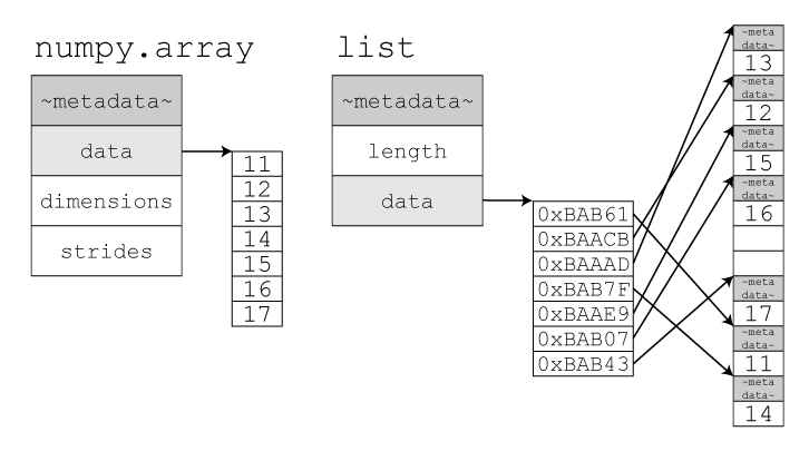
NumPy Arrays and Python Lists Live in Two Separate Worlds
NumPy’s arrays (not to be confused with the core Python
array package) are static arrays. Unlike core Python’s
lists, they do not dynamically resize. Therefore, if you wish to append
to a NumPy array, you must call resize() first. If you
treat this like append() for a Python list, resizing for
each individual append, you will be performing significantly more copies
and memory allocations than a Python list.
The below example sees lists and arrays constructed from
range(100000).
PYTHON
from timeit import timeit
import numpy

N = 100000  # Number of elements in list/array

def list_append():
    ls = []
    for i in range(N):
        ls.append(i)

def array_resize():
    ar = numpy.zeros(1)
    for i in range(1, N):
        ar.resize(i+1)
        ar[i] = i

repeats = 1000
print(f"list_append: {timeit(list_append, number=repeats):.2f}ms")
print(f"array_resize: {timeit(array_resize, number=repeats):.2f}ms")
For Python lists, we’ve seen earlier that list comprehensions are
more efficient, so we prefer to avoid using a large number of
append operations if possible. Similarly, we should try to
avoid resizing NumPy arrays, where the overhead is even higher (5.2x
slower than a list, probably 10x slower than list comprehension).
OUTPUT
list_append: 3.50ms
array_resize: 18.04ms
Another difference, is that NumPy arrays typically require all data to be the same type (and a NumPy type). This enables more efficient access to elements, as they all exist contiguously in memory. In contrast, elements within Python lists can be of any type so the list always stores a pointer to where the element actually exists in memory, rather than the actual element. This has the side effect that if you are converting back and forth between Python lists and NumPy arrays, there is an additional overhead as it’s not as simple as copying a single block of memory.
If you construct a NumPy array from a list containing a complex object, it will store your data as Python types and you won’t be able to take advantage of NumPy’s optimisations.
The below example demonstrates the overhead of mixing Python lists and NumPy functions.
SH
# Python list, numpy.random.choice()
>python -m timeit -s "import numpy; ls = list(range(10000))" "numpy.random.choice(ls)"
1000 loops, best of 5: 267 usec per loop

# NumPy array, numpy.random.choice()
>python -m timeit -s "import numpy; ar = numpy.arange(10000)" "numpy.random.choice(ar)"
50000 loops, best of 5: 4.06 usec per loop
Passing a Python list to numpy.random.choice() is 65.6x
slower than passing a NumPy array. This is the additional overhead of
converting the list to an array. If this function were called multiple
times, it would make sense to transform the list to an array before
calling the function so that overhead is only paid once.
SH
# Python list, Manually select 1 item
>python -m timeit -s "import numpy; ls = list(range(10000))" "ls[numpy.random.randint(len(ls))]"
200000 loops, best of 5: 1.19 usec per loop

# NumPy array, Manually select 1 item
>python -m timeit -s "import numpy; ar = numpy.arange(10000)" "ar[numpy.random.randint(len(ar))]"
200000 loops, best of 5: 1.22 usec per loop
Regardless, for this simple application of
numpy.random.choice(), merely using
numpy.random.randint(len()) is around 4x faster regardless
whether a Python list or NumPy array is used.
With numpy.random.choice() being such a general function
(it has many possible parameters), there is significant internal
branching. If you don’t require this advanced functionality and are
calling a function regularly, it can be worthwhile considering using a
more limited function.
There is however a trade-off, using
numpy.random.choice() can be clearer to someone reading
your code, and is more difficult to use incorrectly.
Array Broadcasting
NumPy arrays support “broadcasting” many mathematical operations or functions. This is a shorthand notation, where the operation/function is applied element-wise without having to loop over the array explicitly:
PYTHON
>>> import numpy as np
>>> ar = np.arange(6)
>>> ar
array([0, 1, 2, 3, 4, 5])
>>> ar + 10
array([10, 11, 12, 13, 14, 15])
>>> ar * 2
array([ 0,  2,  4,  6,  8, 10])
>>> ar**2
array([ 0,  1,  4,  9, 16, 25])
>>> np.exp(ar)
array([  1.        ,   2.71828183,   7.3890561 ,  20.08553692,
54.59815003, 148.4131591 ])If you try the same with Python lists, it will usually fail with an error or give an unexpected result:
PYTHON
>>> ls = list(range(6))
>>> ls + 10
Traceback (most recent call last):
  File "<python-input-8>", line 1, in <module>
    ls + 10
    ~~~^~~~
TypeError: can only concatenate list (not "int") to list
>>> ls * 2
[0, 1, 2, 3, 4, 5, 0, 1, 2, 3, 4, 5]
>>> ls ** 2
Traceback (most recent call last):
  File "<python-input-10>", line 1, in <module>
    ls ** 2
    ~~~^^~~
TypeError: unsupported operand type(s) for ** or pow(): 'list' and 'int'
>>> np.exp(ls)  # works but is slower, because NumPy converts the list into an array first
array([  1.        ,   2.71828183,   7.3890561 ,  20.08553692,
        54.59815003, 148.4131591 ])
However, broadcasting is not just a nicer way to write mathematical expressions—it can also give a significant performance boost: Most modern processors are able to apply one instruction across multiple variables simultaneously, instead of sequentially. (In computer science, this is also referred to as “vectorisation”.) The manner by which NumPy stores data in arrays enables it to vectorise mathematical operations that are broadcast across arrays.
SH
> python -m timeit -s "import numpy; ar = numpy.arange(1)" "ar + 10"
1000000 loops, best of 5: 359 nsec per loop
> python -m timeit -s "import numpy; ar = numpy.arange(10)" "ar + 10"
1000000 loops, best of 5: 362 nsec per loop
> python -m timeit -s "import numpy; ar = numpy.arange(100)" "ar + 10"
1000000 loops, best of 5: 364 nsec per loop
If we were to use a regular for loop, the time to
perform this operation would increase with the length of the array.
However, using NumPy broadcasting we can apply the addition to 1, 10 or
100 elements, all in the same amount of time!
A simple analogy:
If you’re baking cookies, the oven (CPU register) is big enough to operate on multiple cookies (numbers) simultaneously. So whether you bake 1 cookie or 10, it’ll take exactly the same amount of time. However, this requires that the cookies are neatly arranged on a baking tray (in a contiguous chunk of memory).
Basic ints/floats in NumPy arrays are arranged like that, so this works great. In contrast, numbers in a Python list are spread across memory in a fairly complex arrangement, so cannot benefit from this unless you convert them to a NumPy array first.
Earlier it was demonstrated that using core Python methods over a list will outperform a loop, performing the same calculation faster. The below example takes this a step further by demonstrating the calculation of a dot product.
PYTHON
from timeit import timeit

N = 1000000  # Number of elements in list

gen_list = f"ls = list(range({N}))"
gen_array = f"import numpy; ar = numpy.arange({N}, dtype=numpy.int64)"

py_sum_ls = "sum([i*i for i in ls])"
py_sum_ar = "sum(ar*ar)"
np_sum_ar = "numpy.sum(ar*ar)"
np_dot_ar = "numpy.dot(ar, ar)"

repeats = 1000
print(f"python_sum_list: {timeit(py_sum_ls, setup=gen_list, number=repeats):.2f}ms")
print(f"python_sum_array: {timeit(py_sum_ar, setup=gen_array, number=repeats):.2f}ms")
print(f"numpy_sum_array: {timeit(np_sum_ar, setup=gen_array, number=repeats):.2f}ms")
print(f"numpy_dot_array: {timeit(np_dot_ar, setup=gen_array, number=repeats):.2f}ms")
OUTPUT
python_sum_list: 46.93ms
python_sum_array: 33.26ms
numpy_sum_array: 1.44ms
numpy_dot_array: 0.29ms-
python_sum_listuses list comprehension to perform the multiplication, followed by the Python coresum(). This comes out at 46.93ms -
python_sum_arrayinstead directly multiplies the two arrays (taking advantage of NumPy’s vectorisation) but uses the core Pythonsum(), this comes in slightly faster at 33.26ms. -
numpy_sum_arrayagain takes advantage of NumPy’s vectorisation for the multiplication, and additionally uses NumPy’ssum()implementation. These two rounds of vectorisation provide a much faster 1.44ms completion. -
numpy_dot_arrayinstead uses NumPy’sdot()to calculate the dot product in a single operation. This comes out the fastest at 0.29ms, 162x faster thanpython_sum_list.
Parallel NumPy
NumPy can sometimes take advantage of auto parallelisation, particularly on HPC systems.
A small number of functions are backed by BLAS and LAPACK, enabling even greater speedup.
The supported
functions mostly correspond to linear algebra operations like
numpy.dot().
The auto-parallelisation of these functions is hardware-dependent, so you won’t always automatically get the additional benefit of parallelisation. However, HPC systems should be primed to take advantage, so try increasing the number of cores you request when submitting your jobs and see if it improves the performance.
This might be why numpy_dot_array is that much
faster than numpy_sum_array in the previous
example!
Other Libraries That Use NumPy
Across the scientific Python software ecosystem, many domain-specific packages are built on top of NumPy arrays. Similar to the demos above, we can often gain significant performance boosts by using these libraries well.
Challenge: Which Libraries Are You Using Already?
Take a look at the list of libraries on the NumPy website. Are you using any of them already?
If you’ve brought a project you want to work on: Are there areas of the project where you might benefit from adapting one of these libraries instead of writing your own code from scratch?
These libraries could be specific to your area of research; but they could also include packages from other fields that provide tools you need (e.g. statistics or machine learning)!
Which libraries you may use will depend on your research domain; here, we’ll show an example from bioinformatics.
Example: Image Analysis with Shapely
A bioinformatics researcher had a large data set of images of cells. She had already reconstructed the locations of cell walls and various points of interest and needed to identify which points were located in each cell. To do this, she used the Shapely geometry library.
PYTHON
points_per_polygon = {}
for polygon_idx in range(n_polygons):
    current_polygon = polygons.iloc[polygon_idx,:]["geometry"]

    # manually loop over all points, check if polygon contains that point
    out_points = []
    for i in range(n_points):
        current_point = points.iloc[i, :]
        if current_polygon.contains(current_point["geometry"]):
            out_points.append(current_point.name)

    points_per_polygon[polygon_idx] = out_points
For about 500k points and 1000 polygons, the initial version of the code took about 20 hours to run.
Luckily, Shapely is built on top of NumPy, so she was able to apply functions to an array of points instead and wrote an improved version, which took just 20 minutes:
PYTHON
# 1) Extract points and corresponding names as two separate NumPy arrays from a larger data frame
# This will make it easier to apply vectorised functions below
points_array = np.array(points.loc[:,"geometry"])
point_names_array = np.array(points.loc[:,"name"])

points_per_polygon = {}
for polygon_idx in range(n_polygons):
    current_polygon = polygons.iloc[polygon_idx,:]["geometry"]

    # 2) apply `contains` to an array of points, rather than an individual point
    points_in_polygon_idx = current_polygon.contains(points_array)
    # 3) Filter `point_names_array` to get just the names of points contained in the polygon
    points_in_polygon = point_names_array[points_in_polygon_idx]
    # 4) Turn this array into a Python list and store it in output data
    points_per_polygon[polygon_idx] = points_in_polygon.tolist()
To vectorise this efficiently, the logic of the code had to be changed slightly:
- The improved code starts by extracting the
shapely.Points and corresponding point names as two separate NumPy arrays from a larger data frame. - It then passes that array of points to
current_polygon.contains(), which uses vectorisation to speed up the calculation. It returns a NumPy array of booleans (TrueorFalse), describing for eachPointin the input array whether it is contained incurrent_polygon. - This boolean array is then passed
as an index to the
point_names_listarray. This returns a new array with the names of all points that are contained in the polygon (i.e. where the boolean array had the valueTrue). - Finally, the contained points are stored as a Python list. (In this particular case, later parts of the data analysis code expected a list instead of a NumPy array. Since those parts of the code were “fast enough”—remember Donald Knuth’s quote in the earlier episode?—the researcher decided not to spend more time to rewrite them.)
The following code snippet demonstrates how this works for a simplified example.
PYTHON
>>> from shapely import Point, Polygon
>>> import numpy as np
>>> polygon = Polygon([(0,0), (1,0), (1,1), (0,1), (0,0)])
>>> points_array = np.array((Point(0.1, 0.1), Point(0.5, 0.5), Point(2, 2)))
>>> point_names_array = np.array(("P1: Periphery", "P2: Centre", "P3: Outside"))
>>> points_in_polygon_idx = polygon.contains(points_array)
>>> points_in_polygon_idx
array([ True,  True, False])
>>> points_in_polygon = point_names_array[points_in_polygon_idx]
>>> points_in_polygon
array(['P1: Periphery', 'P2: Centre'], dtype='<U13')
>>> points_in_polygon.tolist()
['P1: Periphery', 'P2: Centre']
Using Pandas (Effectively)
Pandas is the most common Python package used for scientific computing when working with tabular data akin to spreadsheets (DataFrames).
Similar to NumPy, Pandas enables greater performance than pure Python implementations when used correctly, however incorrect usage can actively harm performance.
Operating on Rows
Pandas’ methods by default operate on columns. Each column or series can be thought of as a NumPy array, highly suitable for vectorisation.
Following the theme of this episode, iterating over the rows of a
data frame using a for loop is not advised. The pythonic
iteration will be slower than other approaches.
Pandas allows its own methods to be applied to rows in many cases by
passing axis=1, where available these functions should be
preferred over manual loops. Where you can’t find a suitable method,
apply() can be used, which is similar to
map(), to apply your own function to rows.
PYTHON
from timeit import timeit
import pandas
import numpy

N = 100000  # Number of rows in DataFrame

def genDataFrame():
    numpy.random.seed(12)  # Ensure each dataframe is identical
    return pandas.DataFrame(
    {
        "f_vertical": numpy.random.random(size=N),
        "f_horizontal": numpy.random.random(size=N),
        # todo some spurious columns
    })

def pythagoras(row):
    return (row["f_vertical"]**2 + row["f_horizontal"]**2)**0.5

def for_range():
    rtn = []
    df = genDataFrame()
    for row_idx in range(df.shape[0]):
        row = df.iloc[row_idx]
        rtn.append(pythagoras(row))
    return pandas.Series(rtn)

def for_iterrows():
    rtn = []
    df = genDataFrame()
    for row_idx, row in df.iterrows():
        rtn.append(pythagoras(row))
    return pandas.Series(rtn)

def pandas_apply():
    df = genDataFrame()
    return df.apply(pythagoras, axis=1)

repeats = 1000
gentime = timeit(genDataFrame, number=repeats)
print(f"for_range: {timeit(for_range, number=int(repeats/20))*20-gentime:.2f}ms")  # scale with factor 20, otherwise it takes too long
print(f"for_iterrows: {timeit(for_iterrows, number=int(repeats/20))*20-gentime:.2f}ms")
print(f"pandas_apply: {timeit(pandas_apply, number=int(repeats/20))*20-gentime:.2f}ms")
apply() is 4x faster than the two for
approaches, as it avoids the Python for loop.
OUTPUT
for_range: 1582.47ms
for_iterrows: 1677.14ms
pandas_apply: 390.49ms
However, rows don’t exist in memory as arrays (columns do!), so
apply() does not take advantage of NumPy’s vectorisation.
You may be able to go a step further and avoid explicitly operating on
rows entirely by passing only the required columns to NumPy.
Challenge
We can extract the individual columns of the data frame. These are of
the type pandas.Series, which supports array broadcasting,
just like a NumPy array. Instead of using the
pythagoras(row) function, can you write a vectorised
version of this calculation?
PYTHON
def vectorize():
    df = genDataFrame()
    vertical = df["f_vertical"]
    horizontal = df["f_horizontal"]

    # Your code goes here

    return pandas.Series(results)
Once you’ve done that, measure your performance by running
PYTHON
repeats = 1000
gentime = timeit(genDataFrame, number=repeats)
print(f"vectorize: {timeit(vectorize, number=repeats)-gentime:.2f}ms")
What result do you find? Does this match your expectations?
PYTHON
def vectorize():
    df = genDataFrame()
    vertical = df["f_vertical"]
    horizontal = df["f_horizontal"]

    result = numpy.sqrt(vertical**2 + horizontal**2)

    return pandas.Series(result)

print(f"vectorize: {timeit(vectorize, number=repeats)-gentime:.2f}ms")
264x faster than apply(), 1000x faster than the two
for approaches!
vectorize: 1.48msIt won’t always be possible to take full advantage of vectorisation, for example you may have conditional logic.
An alternate approach is converting your DataFrame to a Python
dictionary using to_dict(orient='index'). This creates a
nested dictionary, where each row of the outer dictionary is an internal
dictionary. This can then be processed via list-comprehension:
PYTHON
def to_dict():
    df = genDataFrame()
    df_as_dict = df.to_dict(orient='index')
    return pandas.Series([(r['f_vertical']**2 + r['f_horizontal']**2)**0.5 for r in df_as_dict.values()])

print(f"to_dict: {timeit(to_dict, number=repeats)*10-gentime:.2f}ms")
Whilst still nearly 100x slower than pure vectorisation, it’s twice
as fast as apply().
This is because indexing into Pandas’ Series (rows) is
significantly slower than a Python dictionary. There is a slight
overhead to creating the dictionary (40ms in this example), however the
stark difference in access speed is more than enough to overcome that
cost for any large DataFrame.
PYTHON
from timeit import timeit
import pandas as pandas

N = 100000  # Number of rows in DataFrame

def genInput():
    s = pandas.Series({'a' : 1, 'b' : 2})
    d = {'a' : 1, 'b' : 2}
    return s, d

def series():
    s, _ = genInput()
    for i in range(N):
        y = s['a'] * s['b']

def dictionary():
    _, d = genInput()
    for i in range(N):
        y = d['a'] * d['b']

repeats = 1000
print(f"series: {timeit(series, number=repeats):.2f}ms")
print(f"dictionary: {timeit(dictionary, number=repeats):.2f}ms")
65x slower!
OUTPUT
series: 237.25ms
dictionary: 3.63ms
Filter Early
If you can filter your rows before processing, rather than after, you may significantly reduce the amount of processing and memory used.
- Python is an interpreted language, this adds an additional overhead at runtime to the execution of Python code. Many core Python and NumPy functions are implemented in faster C/C++, free from this overhead.
- NumPy can take advantage of vectorisation to process arrays, which can greatly improve performance.
- Many domain-specific packages are built on top of NumPy and can offer similar performance boosts.
- Pandas’ data tables store columns as arrays, therefore operations applied to columns can take advantage of NumPy’s vectorisation.
Content from Keep Python & Packages up to Date
Last updated on 2025-03-08 | Edit this page
Estimated time: 10 minutes
Overview
Questions
- Why would a newer version of Python or a package be faster?
- Are there any risks to updating Python and packages?
- How can reproducibility be ensured through package upgrades?
Objectives
- Able to explain why using the latest versions of Python and packages is beneficial.
- Able to identify when updating is not possible due to incompatibilities.
- Able to ensure code remains reproducible through package changes.
Introduction
It’s important to use the latest Python wherever feasible. In addition to new features and fixes, much work has been completed over the lifetime of Python 3 to improve the performance of the language.
Python 3.11 is between 10-60% faster than Python 3.10. On average, we measured a 1.25x speedup on the standard benchmark suite.
Future proposals, such as changes to the JIT and GIL will provide further improvements to performance.
Similarly, major packages with a performance focus such as NumPy and Pandas, should be kept up to date for the same reasons.
These improvements are often free, requiring minimal changes to any code (unlike the jump from Python 2 to Python 3).
Performance regressions within major packages should be considered rare, they often track performance alongside their test suites.
Support for older Python versions in the Scientific Python ecosystem
In the last few years, many important packages in the Scientific Python ecosystem have agreed a common policy to support previous versions of Python for 3 years. For example, since October 2024, these packages stopped supporting Python 3.10; so if you are still using Python 3.10 (or even older versions), you’re now losing access to new features and performance improvements in NumPy, SciPy, Matplotlib and many other libraries. Time to update!
However, the more packages and language features your code touches, and the older the Python it currently uses, the greater chance of incompatibilities making it difficult to upgrade.
Similar to optimising, when updating it’s important to have tests in place to validate the correctness of your code before and after changes. An update to a single small dependent package could introduce a breaking change. This could cause your code to crash, or worse subtly change your results.
Updating Python & Packages
This isn’t as relevant if you’re starting from scratch. Simply make sure you’ve installed the latest Python before you start.
If you have been working with an existing Python installation, the upgrade process for Python itself depends on how you installed your current version. (E.g. via conda, official installer from python.org, package manager like Homebrew/apt/yum/…)
For packages you’re using, you can update those with the same package manager you used to installed them:
- via
pip, e.g.pip install --upgrade numpy - via
conda, e.g.conda update <PACKAGE>
- Where feasible, the latest version of Python and packages should be used as they can include significant free improvements to the performance of your code.
- There is a risk that updating Python or packages will not be possible to due to version incompatibilities or will require breaking changes to your code.
- Changes to packages may impact results output by your code, ensure you have a method of validation ready prior to attempting upgrades.
Content from Understanding Latency
Last updated on 2025-05-11 | Edit this page
Estimated time: 30 minutes
Overview
Questions
- Why is it faster to read/write a single 100 MB file, than 100 files of 1 MB each?
- How many orders of magnitude slower are disk accesses than RAM?
- What’s the cost of creating a list?
Objectives
- Able to identify the relationship between different latencies relevant to software.
- Demonstrate how to implement parallel network requests.
- Justify the re-use of existing variables over creating new ones.
Accessing Disk
When reading data from a file, it is first transferred from the disk to the disk cache and then to the RAM (the computer’s main memory, where variables are stored). The latency to access files on disk is another order of magnitude higher than accessing normal variables.
As such, disk accesses benefit from sequential accesses and reading
larger blocks together rather than single variables. Python’s
io package is already buffered, so automatically handles
this for you in the background.
However before a file can be read, the file system on the disk must be polled to transform the file path to its address on disk to initiate the transfer (or throw an exception).
Following the common theme of this episode, accessing randomly scattered files can be significantly slower than accessing a single larger file of the same size. This is because for each file accessed, the file system must be polled to transform the file path to an address on disk. Traditional hard disk drives particularly suffer, as the read head must physically move to locate data.
Hence, it can be wise to avoid storing outputs in many individual files and to instead create a larger output file.
This is even visible outside of your own code. If you try to upload/download 1 GB to HPC. The transfer will be significantly faster, assuming good internet bandwidth, if that’s a single file rather than thousands.
The below example code runs a small benchmark, whereby 10MB is written to disk and read back whilst being timed. In one case this is as a single file, and in the other, 1000 file segments.
PYTHON
import os, time

# Generate 10MB
data_len = 10000000
data = os.urandom(data_len)
file_ct = 1000
file_len = int(data_len/file_ct)
# Write one large file
start = time.perf_counter()
large_file = open("large.bin", "wb")
large_file.write(data)
large_file.close ()
large_write_s = time.perf_counter() - start
# Write multiple small files
start = time.perf_counter()
for i in range(file_ct):
    small_file = open(f"small_{i}.bin", "wb")
    small_file.write(data[file_len*i:file_len*(i+1)])
    small_file.close()
small_write_s = time.perf_counter() - start
# Read back the large file
start = time.perf_counter()
large_file = open("large.bin", "rb")
t = large_file.read(data_len)
large_file.close ()
large_read_s = time.perf_counter() - start
# Read back the small files
start = time.perf_counter()
for i in range(file_ct):
    small_file = open(f"small_{i}.bin", "rb")
    t = small_file.read(file_len)
    small_file.close()
small_read_s = time.perf_counter() - start
# Print Summary
print(f"{1:5d}x{data_len/1000000}MB Write: {large_write_s:.5f} seconds")
print(f"{file_ct:5d}x{file_len/1000}KB Write: {small_write_s:.5f} seconds")
print(f"{1:5d}x{data_len/1000000}MB Read: {large_read_s:.5f} seconds")
print(f"{file_ct:5d}x{file_len/1000}KB Read: {small_read_s:.5f} seconds")
print(f"{file_ct:5d}x{file_len/1000}KB Write was {small_write_s/large_write_s:.1f} slower than 1x{data_len/1000000}MB Write")
print(f"{file_ct:5d}x{file_len/1000}KB Read was {small_read_s/large_read_s:.1f} slower than 1x{data_len/1000000}MB Read")
# Cleanup
os.remove("large.bin")
for i in range(file_ct):
    os.remove(f"small_{i}.bin")
Running this locally, with an SSD I received the following timings.
SH
    1x10.0MB Write: 0.00198 seconds
 1000x10.0KB Write: 0.14886 seconds
    1x10.0MB Read: 0.00478 seconds
 1000x10.0KB Read: 2.50339 seconds
 1000x10.0KB Write was 75.1 slower than 1x10.0MB Write
 1000x10.0KB Read was 523.9 slower than 1x10.0MB Read
Repeated runs show some noise to the timing, however the slowdown is consistently the same order of magnitude slower when split across multiple files.
You might not even be reading 1000 different files. You could be reading the same file multiple times, rather than reading it once and retaining it in memory during execution. An even greater overhead would apply.
Accessing the Network
When transferring files over a network, similar effects apply. There is a fixed overhead for every file transfer (no matter how big the file), so downloading many small files will be slower than downloading a single large file of the same total size.
Because of this overhead, downloading many small files often does not use all the available bandwidth. It may be possible to speed things up by parallelising downloads.
PYTHON
from concurrent.futures import ThreadPoolExecutor, as_completed
from timeit import timeit
import requests  # install with `pip install requests`


def download_file(url, filename):
    response = requests.get(url)
    with open(filename, 'wb') as f:
        f.write(response.content)
    return filename

downloaded_files = []

def sequentialDownload():
    for mass in range(10, 20):
        url = f"https://github.com/SNEWS2/snewpy-models-ccsn/raw/refs/heads/main/models/Warren_2020/stir_a1.23/stir_multimessenger_a1.23_m{mass}.0.h5"
        f = download_file(url, f"seq_{mass}.h5")
        downloaded_files.append(f)

def parallelDownload():
    # Initialise a pool of 6 threads to share the workload
    pool = ThreadPoolExecutor(max_workers=6)
    jobs = []
    # Submit each download to be executed by the thread pool
    for mass in range(10, 20):
        url = f"https://github.com/SNEWS2/snewpy-models-ccsn/raw/refs/heads/main/models/Warren_2020/stir_a1.23/stir_multimessenger_a1.23_m{mass}.0.h5"
        local_filename = f"par_{mass}.h5"
        jobs.append(pool.submit(download_file, url, local_filename))

    # Collect the results (and errors) as the jobs are completed
    for result in as_completed(jobs):
        if result.exception() is None:
            # handle return values of the parallelised function
            f = result.result()
            downloaded_files.append(f)
        else:
            # handle errors
            print(result.exception())

    pool.shutdown(wait=False)


print(f"sequentialDownload: {timeit(sequentialDownload, globals=globals(), number=1):.3f} s")
print(downloaded_files)
downloaded_files = []
print(f"parallelDownload: {timeit(parallelDownload, globals=globals(), number=1):.3f} s")
print(downloaded_files)
Depending on your internet connection, results may vary significantly, but the parallel download will usually be quite a bit faster. Note also that the order in which the parallel downloads finish will vary.
OUTPUT
sequentialDownload: 3.225 s
['seq_10.h5', 'seq_11.h5', 'seq_12.h5', 'seq_13.h5', 'seq_14.h5', 'seq_15.h5', 'seq_16.h5', 'seq_17.h5', 'seq_18.h5', 'seq_19.h5']
parallelDownload: 0.285 s
['par_11.h5', 'par_12.h5', 'par_15.h5', 'par_13.h5', 'par_10.h5', 'par_14.h5', 'par_16.h5', 'par_19.h5', 'par_17.h5', 'par_18.h5']
Latency Overview
Latency can have a big impact on the speed that a program executes, the below graph demonstrates this. Note the log scale!
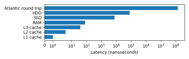
L1/L2/L3 caches are where your most recently accessed variables are stored inside the CPU, whereas RAM is where most of your variables will be found.
The lower the latency typically the higher the effective bandwidth (L1 and L2 cache have 1 TB/s, RAM 100 GB/s, SSDs up to 32 GB/s, HDDs up to 150 MB/s), making large memory transactions even slower.
Memory Allocation is not Free
When a variable is created, memory must be located for it, potentially requested from the operating system. This gives it an overhead versus reusing existing allocations, or avoiding redundant temporary allocations entirely.
Within Python memory is not explicitly allocated and deallocated, instead it is automatically allocated and later “garbage collected”. The costs are still there, this just means that Python programmers have less control over where they occur.
The below implementation of the heat-equation,
reallocates out_grid, a large 2 dimensional (500x500) list
each time update() is called which progresses the
model.
PYTHON
grid_shape = (512, 512)

def update(grid, a_dt):
    x_max, y_max = grid_shape
    out_grid = [[0.0 for x in range(y_max)] * y_max for x in range(x_max)]
    for i in range(x_max):
        for j in range(y_max):
            out_xx = grid[(i-1)%x_max][j] - 2 * grid[i][j] + grid[(i+1)%x_max][j]
            out_yy = grid[i][(j-1)%y_max] - 2 * grid[i][j] + grid[i][(j+1)%y_max]
            out_grid[i][j] = grid[i][j] + (out_xx + out_yy) * a_dt
    return out_grid

def heat_equation(steps):
    x_max, y_max = grid_shape
    grid = [[0.0] * y_max for x in range(x_max)]
    # Init central point to diffuse
    grid[int(x_max/2)][int(y_max/2)] = 1.0
    # Run steps
    for i in range(steps):
        grid = update(grid, 0.1)

heat_equation(100)
Line profiling demonstrates that function takes up over 55 seconds of
the total runtime, with the cost of allocating the temporary
out_grid list to be 39.3% of the total runtime of that
function!
OUTPUT
Total time: 55.4675 s
File: heat_equation.py
Function: update at line 4

Line #      Hits         Time  Per Hit   % Time  Line Contents
==============================================================
     3                                           @profile
     4                                           def update(grid, a_dt):
     5       100        127.7      1.3      0.0      x_max, y_max = grid_shape
     6       100   21822304.9 218223.0     39.3      out_grid = [[0.0 for x in range(y_max)] * y_max for x in range(x_m…
     7     51300       7741.9      0.2      0.0      for i in range(x_max):
     8  26265600    3632718.1      0.1      6.5          for j in range(y_max):
     9  26214400   11207717.9      0.4     20.2              out_xx = grid[(i-1)%x_max][j] - 2 * grid[i][j] + grid[(i+1…
    10  26214400   11163116.5      0.4     20.1              out_yy = grid[i][(j-1)%y_max] - 2 * grid[i][j] + grid[i][(…
    11  26214400    7633720.1      0.3     13.8              out_grid[i][j] = grid[i][j] + (out_xx + out_yy) * a_dt
    12       100         27.8      0.3      0.0      return out_grid
If instead out_grid is double buffered, such that two
buffers are allocated outside the function, which are swapped after each
call to update().
PYTHON
grid_shape = (512, 512)

def update(grid, a_dt, out_grid):
    x_max, y_max = grid_shape
    for i in range(x_max):
        for j in range(y_max):
            out_xx = grid[(i-1)%x_max][j] - 2 * grid[i][j] + grid[(i+1)%x_max][j]
            out_yy = grid[i][(j-1)%y_max] - 2 * grid[i][j] + grid[i][(j+1)%y_max]
            out_grid[i][j] = grid[i][j] + (out_xx + out_yy) * a_dt

def heat_equation(steps):
    x_max, y_max = grid_shape
    grid = [[0.0 for x in range(y_max)] for x in range(x_max)]
    out_grid = [[0.0 for x in range(y_max)] for x in range(x_max)]  # Allocate a second buffer once
    # Init central point to diffuse
    grid[int(x_max/2)][int(y_max/2)] = 1.0
    # Run steps
    for i in range(steps):
        update(grid, 0.1, out_grid)  # Pass the output buffer
        grid, out_grid = out_grid, grid  # Swap buffers

heat_equation(100)
The total time reduces to 34 seconds, reducing the runtime by 39% inline with the removed allocation.
OUTPUT
Total time: 34.0597 s
File: heat_equation.py
Function: update at line 3

Line #      Hits         Time  Per Hit   % Time  Line Contents
==============================================================
     3                                           @profile
     4                                           def update(grid, a_dt, out_grid):
     5       100         43.5      0.4      0.0      x_max, y_max = grid_shape
     6     51300       7965.8      0.2      0.0      for i in range(x_max):
     7  26265600    3569519.4      0.1     10.5          for j in range(y_max):
     8  26214400   11291491.6      0.4     33.2              out_xx = grid[(i-1)%x_max][j] - 2 * grid[i][j] + grid[(i+1…
     9  26214400   11409533.7      0.4     33.5              out_yy = grid[i][(j-1)%y_max] - 2 * grid[i][j] + grid[i][(…
10 26214400 7781156.4 0.3 22.8 out_grid[i][j] = grid[i][j] + (out_xx + out_yy) * a_dt- One large file is preferable to many small files.
- Network requests can be parallelised to reduce the impact of fixed overheads.
- Memory allocation is not free, avoiding destroying and recreating objects can improve performance.
Content from Optimisation Conclusion
Last updated on 2025-05-11 | Edit this page
Estimated time: 5 minutes
Overview
Questions
- What has been learnt about writing performant Python?
Objectives
- Review what has been learnt about writing performant Python
This concludes the optimisation portion of the course.
An overview of how Python operates and the most important practices for achieving performant code have been introduced.
Hopefully with the information from this course you will be in a better position to investigate and optimise the performance of your own code.
This course’s website can be used as a reference manual when profiling your own code.
Your Feedback is Required!
Please complete this Google form to let us know what you think we’ve missed.
Your feedback enables us to improve the course for future attendees!
- Using Python Language Features and the Standard Library
- Python is an interpreted language. This adds an additional overhead at runtime to the execution of Python code. Many core Python functions are implemented in faster C/C++, free from this overhead.
- Where possible, use built-in functions (like
sum(),min()ormax()), language features (like list comprehensions) and standard library functionality (likestr.split()) instead of re-inventing the wheel. This makes your code more readable and is often more performant.
- Data Structures & Algorithms
- List comprehension should be preferred when constructing lists.
- Where appropriate, Tuples and Generator functions should be preferred over Python lists.
- Dictionaries and sets are appropriate for storing a collection of unique data with no intrinsic order for random access.
- When used appropriately, dictionaries and sets are significantly faster than lists.
- If searching a list or array is required, it should be sorted and
searched using
bisect_left()(binary search).
- Minimise Python Written
- Like many core Python functions, NumPy functions are implemented in faster C/C++.
- Additionally, NumPy can take advantage of vectorisation to process arrays, which can greatly improve performance.
- Pandas’ data tables store columns as arrays, therefore operations applied to columns can take advantage of NumPys vectorisation.
- Newer is Often Faster
- Where feasible, the latest version of Python and packages should be used as they can include significant free improvements to the performance of your code.
- There is a risk that updating Python or packages will not be possible to due to version incompatibilities or will require breaking changes to your code.
- Changes to packages may impact results output by your code, ensure you have a method of validation ready prior to attempting upgrades.
- How Latency Affects Performance
- One large file is preferable to many small files.
- Network requests can be parallelised to reduce the impact of fixed overheads.
- Memory allocation is not free, avoiding destroying and recreating objects can improve performance.